17  Linking Sensor Streams

Each element in a Tandem facility can have sensor streams attached to it, named time-series channels that report temperature, CO₂, occupancy, energy consumption, or whatever the building management system sends. Because streams are keyed to the same objectId that getObjectTree() and getData() use, joining live sensor data to BIM metadata is just a regular table join.

This chapter uses the facility set up in AutoDesk Tandem Overview.

17.1 Listing Streams for a Facility

library(AutoDeskR)
library(httr2)
library(dplyr)

resp       <- getToken(id     = Sys.getenv("client_id"),
                       secret = Sys.getenv("client_secret"),
                       scope  = "data:read")
myToken    <- resp$content$access_token
facilityId <- "urn:adsk.dtdm:facility.abc123def456"

streams_resp <- request(
  paste0("https://tandem.autodesk.com/api/v1/twins/", facilityId, "/streams")
) |>
  req_auth_bearer_token(myToken) |>
  req_perform()

streams <- resp_body_json(streams_resp)

streams_df <- lapply(streams, function(s) {
  data.frame(stream_id    = s$id,
             display_name = s$displayName,
             element_id   = s$elementId,   # objectId of the attached model element
             unit         = s$unit,
             last_reading = s$lastValue,
             stringsAsFactors = FALSE)
}) |> do.call(what = rbind)

streams_df
#>            stream_id    display_name element_id  unit last_reading
#> 1  strm:temp-hvac-l2  HVAC Temp L2          42    °C         22.4
#> 2  strm:co2-office-3  CO₂ Office 3         108   ppm        623.0
#> 3  strm:occ-lobby     Lobby Occupancy        15  pers         14.0
#> 4  strm:energy-main   Main Energy          201   kWh       8412.5

Important

Replace before running: facilityId ("urn:adsk.dtdm:facility.abc123def456") with your own Tandem facility URN, and set client_id/client_secret in ~/.Renviron. The stream IDs above are illustrative.

17.2 Fetching Time-Series Readings

Request a time window using ISO 8601 timestamps as query parameters:

streamId   <- "strm:temp-hvac-l2"
end_time   <- Sys.time()
start_time <- end_time - 86400   # last 24 hours

readings_resp <- request(
  paste0("https://tandem.autodesk.com/api/v1/twins/",
         facilityId, "/streams/", streamId)
) |>
  req_url_query(
    start = format(start_time, "%Y-%m-%dT%H:%M:%SZ", tz = "UTC"),
    end   = format(end_time,   "%Y-%m-%dT%H:%M:%SZ", tz = "UTC")
  ) |>
  req_auth_bearer_token(myToken) |>
  req_perform()

readings <- resp_body_json(readings_resp)

readings_df <- data.frame(
  timestamp = as.POSIXct(vapply(readings$values, `[[`, character(1), "t"),
                          format = "%Y-%m-%dT%H:%M:%SZ", tz = "UTC"),
  value     = vapply(readings$values, `[[`, numeric(1), "v"),
  stringsAsFactors = FALSE
)

head(readings_df)
#>             timestamp value
#> 1 2026-04-23 06:00:00  21.8
#> 2 2026-04-23 06:15:00  22.1
#> 3 2026-04-23 06:30:00  22.4

17.3 Plotting Readings

ggplot(readings_df, aes(x = timestamp, y = value)) +
  geom_line(colour = "#367ABF", linewidth = 0.8) +
  geom_ribbon(aes(ymin = value - 0.5, ymax = value + 0.5),
              fill = "#367ABF", alpha = 0.15) +
  labs(title    = "HVAC Temperature — Level 2",
       subtitle = "Last 24 hours",
       x = NULL, y = "Temperature (°C)") +
  theme_minimal()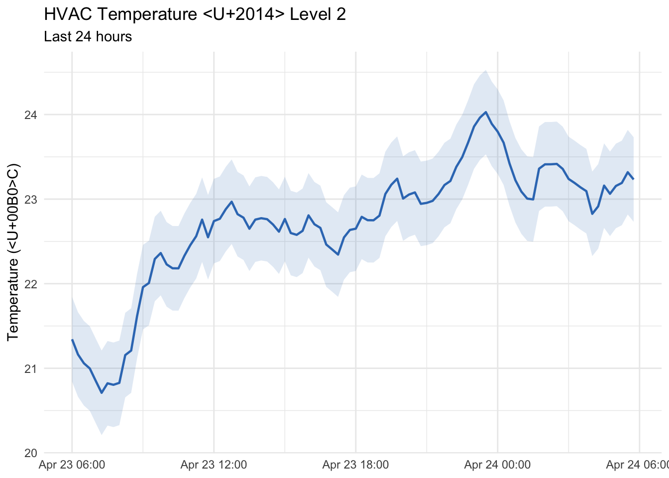

Note

Representative result. This chart and the multi-stream overview below are drawn from synthetic readings so they render without a live Tandem connection. The same plotting code produces the same charts from your facility’s real streams.

17.4 Joining Sensor Data to Model Metadata

element_id in the streams response equals objectid from getData(). A left join links live readings to layer, classification, and any custom attributes:

# props_df from the Layer Structure Analysis chapter

joined <- streams_df |>
  inner_join(props_df |> select(objectid, layer),
             by = c("element_id" = "objectid"))

joined
#>            stream_id    display_name element_id   unit layer
#> 1  strm:temp-hvac-l2  HVAC Temp L2          42    °C  M-HVAC
#> 3  strm:occ-lobby     Lobby Occupancy        15  pers A-LBBY

17.5 Fetching All Streams at Once

Loop over the stream list to build a single tidy data frame of all readings:

all_readings <- lapply(streams_df$stream_id, function(sid) {
  resp <- request(
    paste0("https://tandem.autodesk.com/api/v1/twins/",
           facilityId, "/streams/", sid)
  ) |>
    req_url_query(
      start = format(start_time, "%Y-%m-%dT%H:%M:%SZ", tz = "UTC"),
      end   = format(end_time,   "%Y-%m-%dT%H:%M:%SZ", tz = "UTC")
    ) |>
    req_auth_bearer_token(myToken) |>
    req_perform()
  readings <- resp_body_json(resp)
  data.frame(stream_id = sid,
             timestamp = as.POSIXct(
               vapply(readings$values, `[[`, character(1), "t"),
               format = "%Y-%m-%dT%H:%M:%SZ", tz = "UTC"),
             value     = vapply(readings$values, `[[`, numeric(1), "v"),
             stringsAsFactors = FALSE)
}) |> do.call(what = rbind)

# Join display names and units
all_readings <- all_readings |>
  left_join(streams_df |> select(stream_id, display_name, unit),
            by = "stream_id")

17.6 Multi-Stream Overview Plot

ggplot(all_readings, aes(x = timestamp, y = value, colour = display_name)) +
  geom_line(linewidth = 0.7) +
  facet_wrap(~ paste0(display_name, " (", unit, ")"),
             scales = "free_y", ncol = 2) +
  labs(title = "All Sensor Streams — Last 24 Hours",
       x = NULL, y = NULL) +
  theme_minimal() +
  theme(legend.position = "none")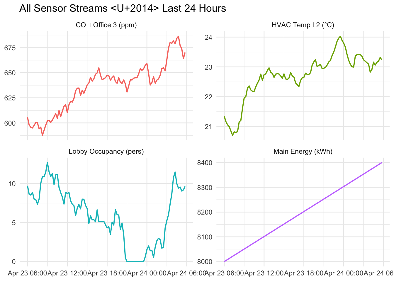

The all_readings data frame feeds directly into the interactive Shiny dashboard in Live Dashboards.