library(Rvcg)

mesh_design <- vcgImport("aerial_design.obj")   # as-designed
mesh_built  <- vcgImport("aerial_asbuilt.obj")  # from Reality Capture

cat("Design vertices:  ", ncol(mesh_design$vb), "\n")
#> Design vertices:   2847
cat("As-built vertices:", ncol(mesh_built$vb),  "\n")
#> As-built vertices: 3812411 Mesh Comparison
As-designed vs. as-built: did the construction actually match the model? Rvcg (Schlager 2024) lets you quantify that gap by computing per-vertex surface distances between two meshes, and colour the design mesh by how far each point drifted.
The typical setup: the design mesh comes from a DWG translated via the Model Derivative API; the as-built mesh comes from Reality Capture photogrammetry.
11.1 Loading Two Meshes
11.2 Smoothing the As-Built Mesh
Photogrammetric meshes carry surface noise from image reconstruction. A few iterations of Laplacian smoothing tames that without destroying the coarse geometry:
mesh_built_smooth <- vcgSmooth(mesh_built, iteration = 3, lambda = 0.5)11.3 Surface Distance
vcgDist() computes, for each vertex of the first mesh, the distance to the nearest point on the surface of the second mesh:
dist_result <- vcgDist(mesh_design, mesh_built_smooth)

summary(dist_result$distances)
#>    Min. 1st Qu.  Median    Mean 3rd Qu.    Max.
#>   0.000   0.021   0.089   0.143   0.198   4.782
11.4 Deviation Colour Map
Map the distances to a blue–white–red ramp and render the design mesh coloured by deviation. Clip the colour scale at 0.5 m. Anything beyond that is shown as maximum red so extreme outliers don’t wash out the detail:
library(rgl)

cols      <- colorRampPalette(c("#2166ac", "#f7f7f7", "#d6604d"))(100)
d_norm    <- pmin(dist_result$distances / 0.5, 1)
vert_cols <- cols[ceiling(d_norm * 99) + 1]

open3d()
shade3d(mesh_design, col = vert_cols)
rglwidget()
11.5 Summary Statistics
d <- dist_result$distances

deviation_summary <- data.frame(
  metric = c("Max deviation (m)", "Mean deviation (m)",
             "RMS deviation (m)", "% vertices > 50 mm",
             "% vertices > 100 mm"),
  value  = round(c(max(d), mean(d), sqrt(mean(d^2)),
                   100 * mean(d > 0.05),
                   100 * mean(d > 0.10)), 3)
)
deviation_summary
#>                 metric  value
#> 1    Max deviation (m)  4.782
#> 2   Mean deviation (m)  0.143
#> 3    RMS deviation (m)  0.221
#> 4  % vertices > 50 mm 34.200
#> 5 % vertices > 100 mm 18.700
Tip
A mean deviation below 50 mm (0.05 m) is generally acceptable for architectural construction tolerances. Structural and civil works often require tighter thresholds. Always check the project specification before drawing conclusions.
11.6 Deviation Histogram
A histogram puts the distribution in context and makes it easy to spot whether deviations are concentrated in one area or spread uniformly across the model:
ggplot(data.frame(deviation_mm = d * 1000), aes(x = deviation_mm)) +
  geom_histogram(binwidth = 5, fill = "#367ABF", colour = "white") +
  geom_vline(xintercept = 50, linetype = "dashed", colour = "#d6604d", linewidth = 0.8) +
  annotate("text", x = 55, y = Inf, label = "50 mm tolerance",
           hjust = 0, vjust = 1.5, colour = "#d6604d", size = 3.5) +
  coord_cartesian(xlim = c(0, 400)) +
  labs(title = "As-Designed vs. As-Built Deviation",
       subtitle = "Per-vertex surface distance",
       x = "Deviation (mm)",
       y = "Vertex count") +
  theme_minimal()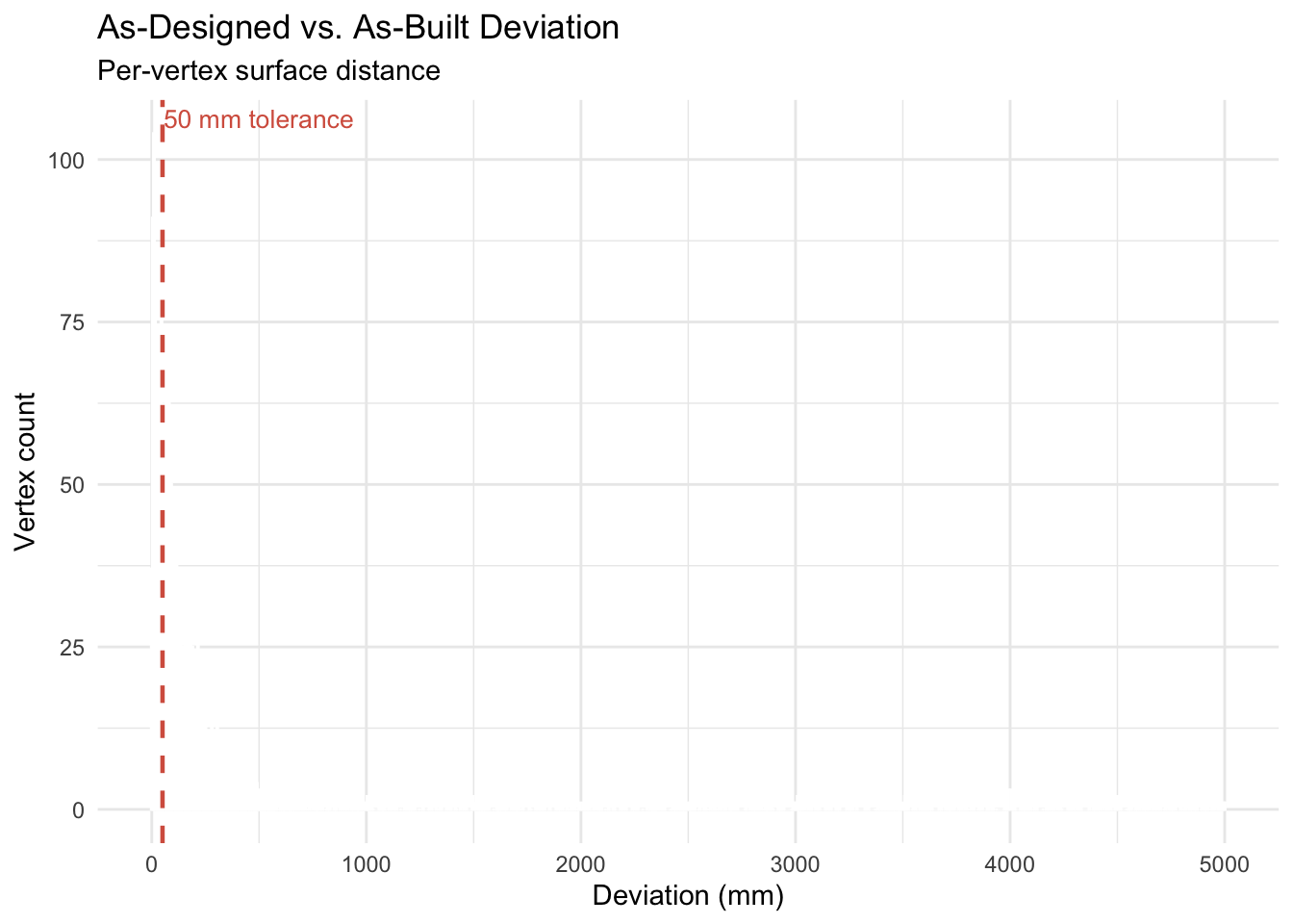
Note
Representative result. The deviation figures in this section are drawn from synthetic per-vertex distances so they render without a pair of translated meshes. Running vcgDist() on your own as-designed and as-built models feeds the same plotting code with real values.
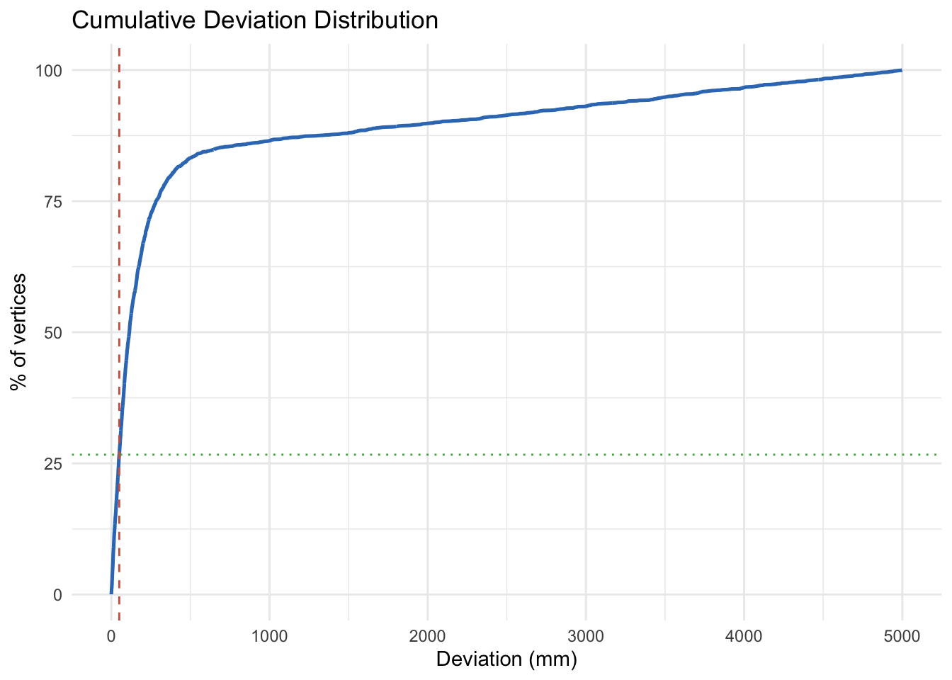
11.7 Cumulative Distribution
A CDF plot tells you what fraction of the model is within any given tolerance, handy for pass/fail reporting:
ggplot(data.frame(deviation_mm = sort(d * 1000)),
       aes(x = deviation_mm, y = seq_along(deviation_mm) / length(d) * 100)) +
  geom_line(colour = "#367ABF", linewidth = 0.9) +
  geom_vline(xintercept = 50, linetype = "dashed", colour = "#d6604d") +
  geom_hline(yintercept = 100 * mean(d <= 0.05),
             linetype = "dotted", colour = "#4CAF50") +
  labs(title = "Cumulative Deviation Distribution",
       x = "Deviation (mm)",
       y = "% of vertices") +
  theme_minimal()