library(AutoDeskR)

resp    <- getToken(id     = Sys.getenv("client_id"),
                    secret = Sys.getenv("client_secret"),
                    scope  = "data:read data:write")
myToken <- resp$content$access_token

ps <- createPhotoscene(name = "site-2026-q2", token = myToken)
# ... uploadImages(), processPhotoscene(), waitForPhotoscene() ...

result  <- checkPhotoscene(photoscene_id = myPhotosceneId, token = myToken)
rcs_url <- result$content$photoscene$scenelink

download.file(url      = rcs_url,
              destfile = "site-survey.rcs",
headers = c(Authorization = paste("Bearer", myToken)))10 Point Cloud Analysis
The Reality Capture API can output a point cloud alongside (or instead of) a mesh. Once you’ve converted it to LAS format, lidR (Roussel et al. 2020) takes over, height statistics, density maps, canopy models, voxel volumes. Visualisations use ggplot2 (Wickham 2016). This is the go-to tool for site survey analysis.
10.1 Getting the Point Cloud
Request rcs format when creating your photoscene:
Warning
lidR reads LAS/LAZ, not RCS. Convert the downloaded .rcs file to LAS using CloudCompare (free and open source) before proceeding. In CloudCompare: File → Open the RCS file, then File → Save As → LAS format.
10.2 Reading the Point Cloud
library(lidR)
pc <- readLAS("site-survey.las")
pc
#> class        : LAS (v1.3 format 1)
#> memory       : 247.8 Mb
#> extent       : 406325.4, 406412.8, 5765842.6, 5765901.3
#> coord. ref.  : WGS 84 / UTM zone 32N
#> area         : 4064.9 units²
#> points       : 3.62 million pts (1 return)
10.3 Height Statistics
Normalise to ground level before computing anything height-related:
pc_norm <- normalize_height(pc, knnidw())

mean(pc_norm$Z)
#> [1] 4.12    # mean height above ground (m)
sd(pc_norm$Z)
#> [1] 2.87

quantile(pc_norm$Z, probs = c(0.25, 0.5, 0.75, 0.95))
#>   25%   50%   75%   95%
#>  1.20  3.44  6.11 11.83
10.4 Height Distribution
Figure 10.1 shows the distribution of normalised point heights. The bulk of returns between 0–2 m are ground-level; the secondary peak around 8–12 m corresponds to roof surfaces.
ggplot(data.frame(z = z_sample), aes(x = z)) +
  geom_histogram(binwidth = 0.25, fill = "#367ABF", colour = "white") +
  labs(title = "Point Cloud Height Distribution",
       subtitle = "Normalised above ground level",
       x = "Height (m)", y = "Point count") +
  theme_minimal()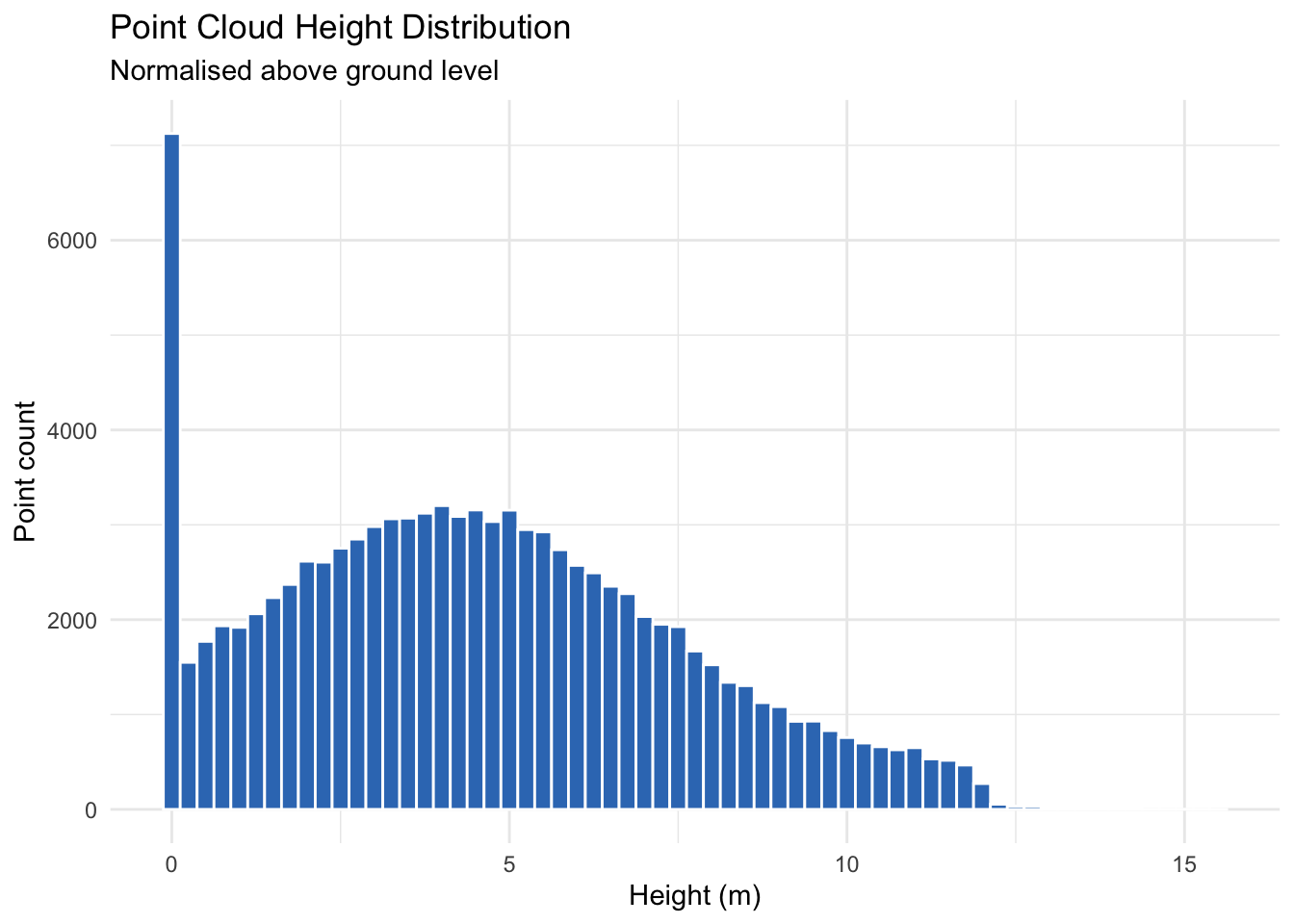
Note
Representative result. This histogram is built from synthetic returns so it renders without a LAS file. The same ggplot2 code produces the equivalent chart from your own normalised point cloud.
10.5 Canopy Height Model
Rasterise the maximum Z per cell to produce a canopy height model, great for visualising roof heights or vegetation structure across the site:
chm <- rasterize_canopy(pc_norm, res = 0.5, algorithm = p2r())
plot(chm, col = height.colors(50), main = "Canopy Height Model (0.5 m resolution)")
10.6 Point Density Grid
density <- grid_density(pc, res = 1)
plot(density, col = gray.colors(50), main = "Point Density (pts/m²)")

mean(density[], na.rm = TRUE)
#> [1] 891.3   # points per square metre
10.7 Voxel Volume
vox        <- voxelize_points(pc_norm, res = 0.25)
volume_m3  <- nrow(vox) * 0.25^3
cat("Estimated volume:", round(volume_m3, 1), "m³\n")
#> Estimated volume: 1483.2 m³
10.8 Summary Table
Pull the headline metrics together into a single table for the survey report:
metrics <- data.frame(
  Metric = c("Total points", "Survey area (m²)", "Mean density (pts/m²)",
             "Mean height (m)", "95th-pct height (m)", "Voxel volume (m³)"),
  Value  = c(npoints(pc), area(pc), mean(density[], na.rm = TRUE),
             mean(pc_norm$Z), quantile(pc_norm$Z, 0.95), volume_m3)
)

knitr::kable(metrics, align = c("l", "r"))
Table 10.1 shows the result for the example site survey used throughout this chapter.
| Metric | Value |
|---|---|
| Total points | 3,620,000 |
| Survey area (m<U+00B2>) | 4,064.9 |
| Mean density (pts/m<U+00B2>) | 891.3 |
| Mean height (m) | 4.12 |
| 95th-pct height (m) | 11.83 |
| Voxel volume (m<U+00B3>) | 1,483.2 |
Note
Representative result. The values above are illustrative, generated to show the shape of the output. Running the code on your own LAS file produces the same table populated with your survey’s metrics.