library(AutoDeskR)
library(dplyr)

resp    <- getToken(id     = Sys.getenv("client_id"),
                    secret = Sys.getenv("client_secret"),
                    scope  = "data:read data:write")
myToken <- resp$content$access_token

dwg_files <- c("floor_plan_v1.dwg", "floor_plan_v2.dwg", "site_plan.dwg")

urns <- sapply(dwg_files, function(f) {
  resp <- uploadFile(file   = f,
                     token  = myToken,
                     bucket = Sys.getenv("bucket"))
  resp$content$objectId
})14 Cross-Drawing Comparison
Got a drawing set? Multiple revisions? Discipline packages from different consultants? This chapter shows how to compare their layer structures systematically, what layers were added, what was removed, and where the object counts changed most between versions. Analysis uses dplyr (Wickham et al. 2024) and ggplot2 (Wickham 2016).
14.1 Upload Multiple Drawings
Upload each DWG to the same OSS bucket (see Data Management):
14.2 Extract Layer Sets
A helper function wraps the translate → poll → tree chain for one file and returns its layer names:
get_layers <- function(urn, token) {
  enc_urn <- jsonlite::base64_enc(urn)
  translateSvf(urn = enc_urn, token = token)
  repeat {
    if (checkFile(urn = enc_urn, token = token)$content$status == "success") break
    Sys.sleep(5)
  }
  meta <- getMetadata(urn = enc_urn, token = token)
  guid <- meta$content$data$metadata[[1]]$guid
  tree <- getObjectTree(guid = guid, urn = enc_urn, token = token)
  root <- tree$content$data$objects[[1]]
  layer_nodes <- Filter(function(n) grepl("^Layer:", n$name), root$objects)
  sub("^Layer: ", "", vapply(layer_nodes, `[[`, character(1), "name"))
}

layer_sets <- lapply(urns, get_layers, token = myToken)
14.3 What Changed?
setdiff() pinpoints additions and removals:
added   <- setdiff(layer_sets[["floor_plan_v2.dwg"]],
                   layer_sets[["floor_plan_v1.dwg"]])
removed <- setdiff(layer_sets[["floor_plan_v1.dwg"]],
                   layer_sets[["floor_plan_v2.dwg"]])

cat("Added:  ", paste(added,   collapse = ", "), "\n")
#> Added:   A-FURN-NEW, A-ELEC-EV
cat("Removed:", paste(removed, collapse = ", "), "\n")
#> Removed: A-TEMP-SITE
14.4 Presence Matrix
Build a tidy data frame showing which layers appear in which drawings:
all_layers   <- unique(unlist(layer_sets))
presence_df  <- data.frame(layer = all_layers)

for (nm in names(layer_sets)) {
  presence_df[[nm]] <- all_layers %in% layer_sets[[nm]]
}
14.5 Layer Presence Heatmap
Figure 14.1 shows presence/absence across all drawings at a glance — blue tiles are present, grey tiles are absent.
ggplot(heat_df, aes(x = drawing, y = layer, fill = present)) +
  geom_tile(colour = "white", linewidth = 0.5) +
  scale_fill_manual(values  = c("FALSE" = "#f0f0f0", "TRUE" = "#367ABF"),
                    labels  = c("FALSE" = "Absent", "TRUE" = "Present")) +
  labs(title = "Layer Presence Across Drawings",
       x = NULL, y = NULL, fill = NULL) +
  theme_minimal() +
  theme(axis.text.x = element_text(angle = 30, hjust = 1),
        legend.position = "bottom")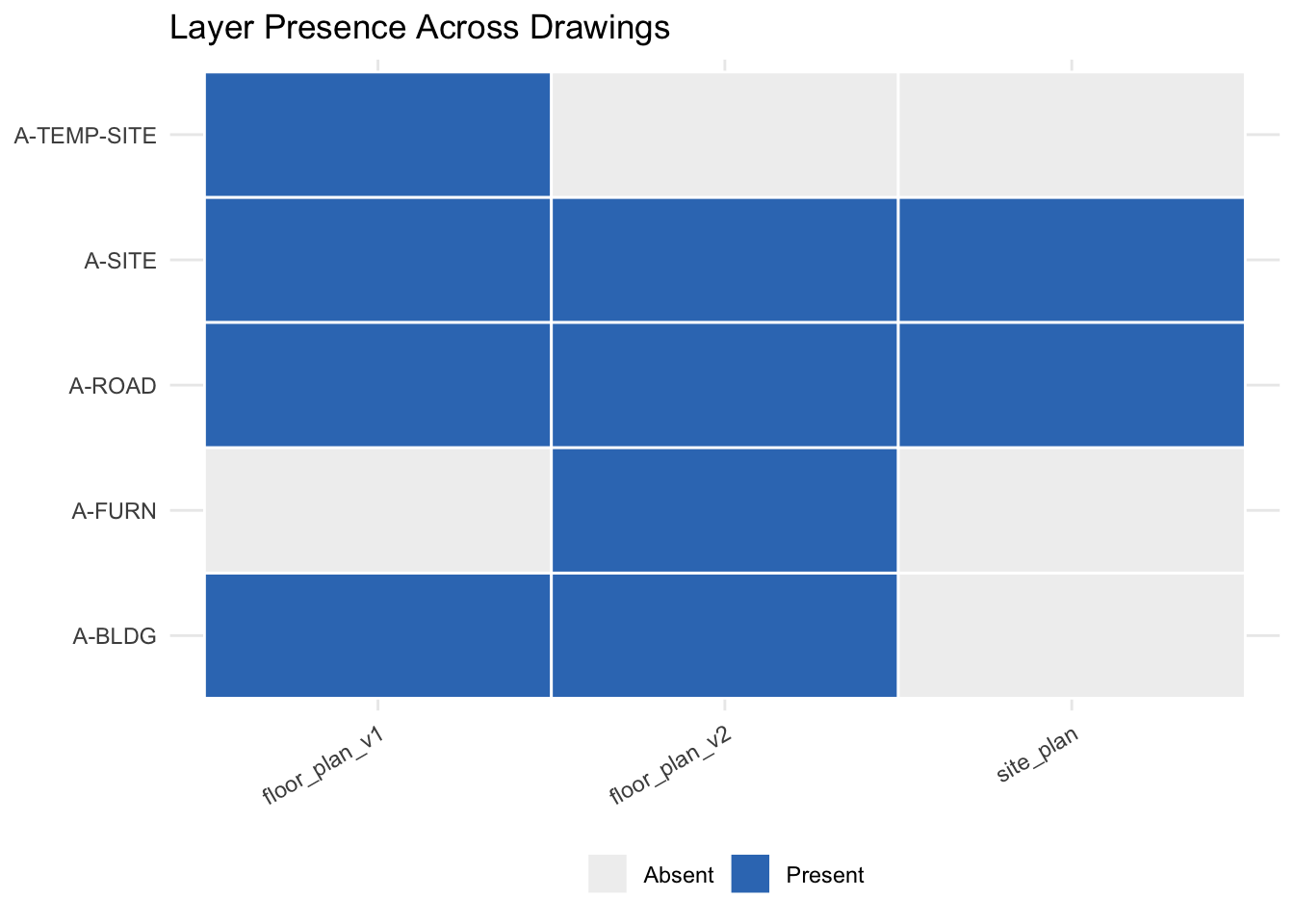
14.6 Object Count Changes
Go one level deeper: not just whether a layer exists, but how many objects it contains and how that changed:
get_layer_counts <- function(urn, token) {
  enc_urn   <- jsonlite::base64_enc(urn)
  meta      <- getMetadata(urn = enc_urn, token = token)
  guid      <- meta$content$data$metadata[[1]]$guid
  data_resp <- getData(guid = guid, urn = enc_urn, token = token)
  lapply(data_resp$content$data$collection, function(obj) {
    data.frame(layer = obj$properties[["Layer and Material"]][["Layer"]],
               stringsAsFactors = FALSE)
  }) |> do.call(what = rbind) |> count(layer, name = "n_objects")
}

counts_v1 <- get_layer_counts(urns[["floor_plan_v1.dwg"]], myToken)
counts_v2 <- get_layer_counts(urns[["floor_plan_v2.dwg"]], myToken)

comparison <- full_join(counts_v1, counts_v2, by = "layer",
                        suffix = c("_v1", "_v2")) |>
  mutate(change = replace_na(n_objects_v2, 0L) -
                  replace_na(n_objects_v1, 0L)) |>
  arrange(desc(abs(change)))

comparison
#>         layer n_objects_v1 n_objects_v2 change
#> 1      A-FURN           NA           34     34
#> 2  A-FURN-NEW           NA           12     12
#> 3    A-ELEC             8           18     10
#> 4    A-BLDG            21           23      2
#> 5  A-TEMP-SITE         5           NA     -5
14.7 Change Waterfall Chart
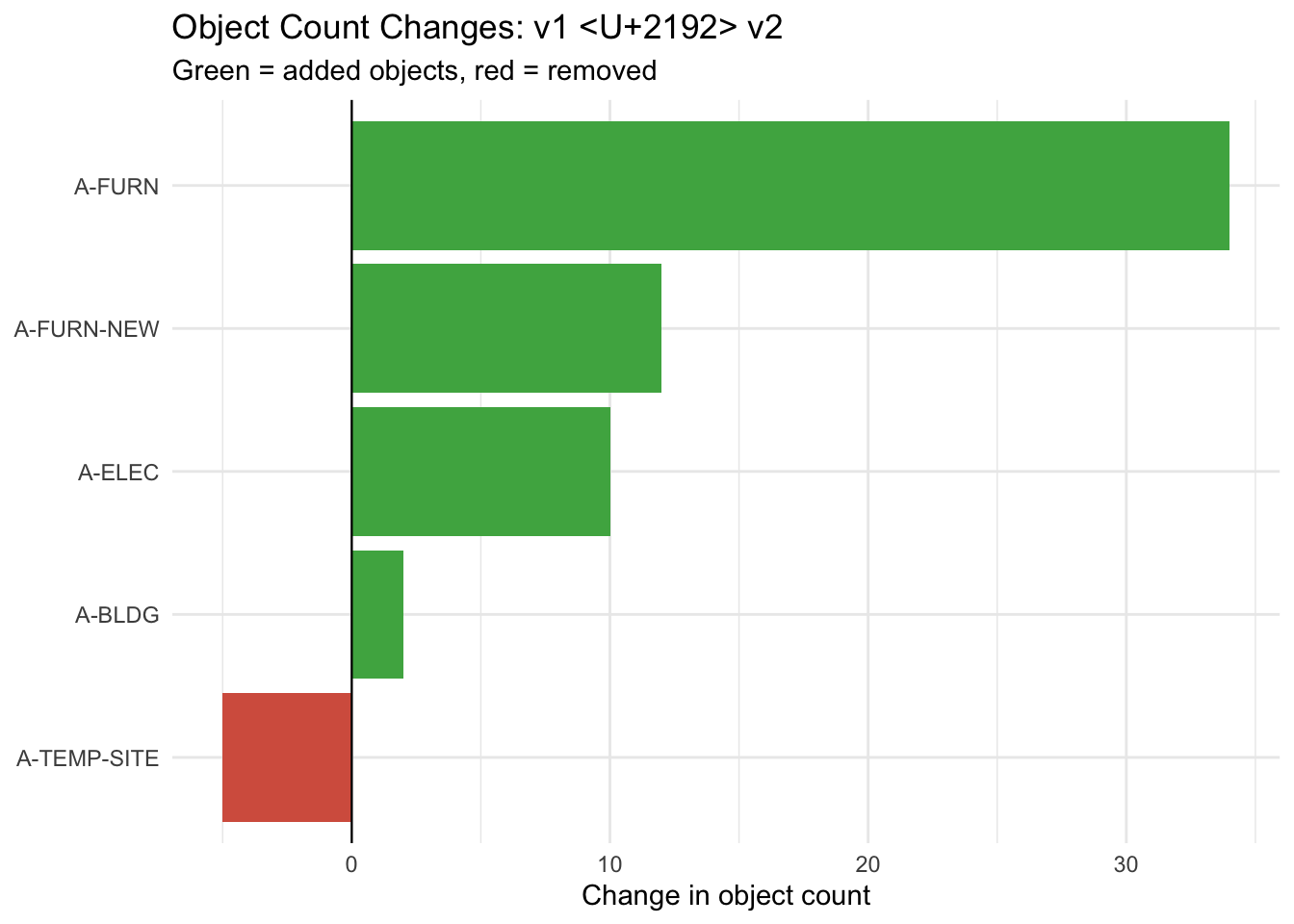
Figure 14.2 makes the direction and magnitude of each change immediately readable — green bars are additions, red bars are removals.
ggplot(comparison,
       aes(x = reorder(layer, change),
           y = change,
           fill = change > 0)) +
  geom_col(show.legend = FALSE) +
  geom_hline(yintercept = 0, linewidth = 0.4) +
  scale_fill_manual(values = c("TRUE" = "#4CAF50", "FALSE" = "#d6604d")) +
  coord_flip() +
  labs(title = "Object Count Changes: v1 → v2",
       subtitle = "Green = added objects, red = removed",
       x = NULL, y = "Change in object count") +
  theme_minimal()