12  Layer Structure Analysis

Every DWG and DXF file organises its geometry into named layers. Unlock those layers through the Model Derivative API and you’ve got a structured dataset ready for dplyr. This chapter extracts per-layer element counts and areas and charts them — no CAD software required.

The data flows like this:

flowchart LR
  A[aerial.dwg] --> B[translateSvf]
  B --> C[getObjectTree\nlayer hierarchy]
  C --> D[getData\nbounding boxes + properties]
  D --> E[dplyr\ngroup_by layer]
  E --> F[ggplot2\nbar chart]

12.1 Prerequisites

install.packages(c("dplyr", "ggplot2"))

12.2 Authenticate and Translate

SVF format is what unlocks metadata access — translate first, then query:

library(AutoDeskR)
library(dplyr)

resp     <- getToken(id     = Sys.getenv("client_id"),
                     secret = Sys.getenv("client_secret"),
                     scope  = "data:read data:write")
myToken  <- resp$content$access_token

myEncodedUrn <- jsonlite::base64_enc(Sys.getenv("urn"))
translateSvf(urn = myEncodedUrn, token = myToken)

repeat {
  status <- checkFile(urn = myEncodedUrn, token = myToken)
  if (status$content$status == "success") break
  Sys.sleep(5)
}

resp_meta <- getMetadata(urn = myEncodedUrn, token = myToken)
myGuid    <- resp_meta$content$data$metadata[[1]]$guid

12.3 The Object Tree

getObjectTree() returns the model hierarchy. In a DWG, the root node’s children are the layers:

tree_resp <- getObjectTree(guid = myGuid, urn = myEncodedUrn, token = myToken)
root      <- tree_resp$content$data$objects[[1]]

root$objects[[1]]
#> $objectid [1] 2
#> $name     [1] "Layer: A-SITE"
#> $objects       # geometry objects on this layer

12.4 Flatten the Tree

A small recursive helper turns the nested list into a tidy data frame — one row per leaf object:

flatten_tree <- function(node, parent_layer = NA_character_) {
  is_layer   <- grepl("^Layer:", node$name)
  layer_name <- if (is_layer) sub("^Layer: ", "", node$name) else parent_layer
  if (is.null(node$objects)) {
    return(data.frame(objectid = node$objectid,
                      name     = node$name,
                      layer    = layer_name,
                      stringsAsFactors = FALSE))
  }
  do.call(rbind, lapply(node$objects, flatten_tree, parent_layer = layer_name))
}

tree_df <- flatten_tree(root)
head(tree_df)
#>   objectid              name   layer
#> 1        5  Polyline (closed)  A-SITE
#> 2        6  Polyline (closed)  A-SITE
#> 3       12              Line  A-BLDG

12.5 Extract Properties with getData()

getData() returns the full property set for every object — including bounding box coordinates:

data_resp  <- getData(guid = myGuid, urn = myEncodedUrn, token = myToken)
collection <- data_resp$content$data$collection

props_df <- lapply(collection, function(obj) {
  geom <- obj$properties$Geometry
  data.frame(
    objectid = obj$objectid,
    layer    = obj$properties[["Layer and Material"]][["Layer"]],
    bb_min_x = geom[["Bounding Box Min X"]],
    bb_min_y = geom[["Bounding Box Min Y"]],
    bb_max_x = geom[["Bounding Box Max X"]],
    bb_max_y = geom[["Bounding Box Max Y"]],
    stringsAsFactors = FALSE
  )
}) |> do.call(what = rbind)

props_df <- props_df |>
  mutate(bb_area = (bb_max_x - bb_min_x) * (bb_max_y - bb_min_y))

Warning

Complex DWGs can return thousands of objects from getData(). For large files, pre-filter the object tree to the layers you care about before calling it to keep response sizes manageable.

12.6 Summarise by Layer

layer_summary <- props_df |>
  group_by(layer) |>
  summarise(n_objects  = n(),
            total_area = sum(bb_area, na.rm = TRUE),
            mean_area  = mean(bb_area, na.rm = TRUE),
            .groups    = "drop") |>
  arrange(desc(total_area))

layer_summary
#> # A tibble: 8 × 4
#>   layer    n_objects total_area mean_area
#>   <chr>        <int>      <dbl>     <dbl>
#> 1 A-SITE          34    156823.    4612.
#> 2 A-BLDG          21     89341.    4254.
#> 3 A-ROAD          12     43218.    3601.
#> 4 A-HATCH          8     12044.    1506.
#> 5 A-TEXT          47      4831.     103.

12.7 Area by Layer — Bar Chart

Warning: package 'ggplot2' was built under R version 4.4.3

ggplot(layer_summary,
       aes(x = reorder(layer, total_area), y = total_area / 1000)) +
  geom_col(fill = "#367ABF") +
  geom_text(aes(label = round(total_area / 1000, 1)),
            hjust = -0.1, size = 3.2) +
  coord_flip() +
  labs(title = "Total Bounding-Box Area by Layer",
       subtitle = "aerial.dwg",
       x = NULL, y = "Area (thousands of drawing units²)") +
  theme_minimal()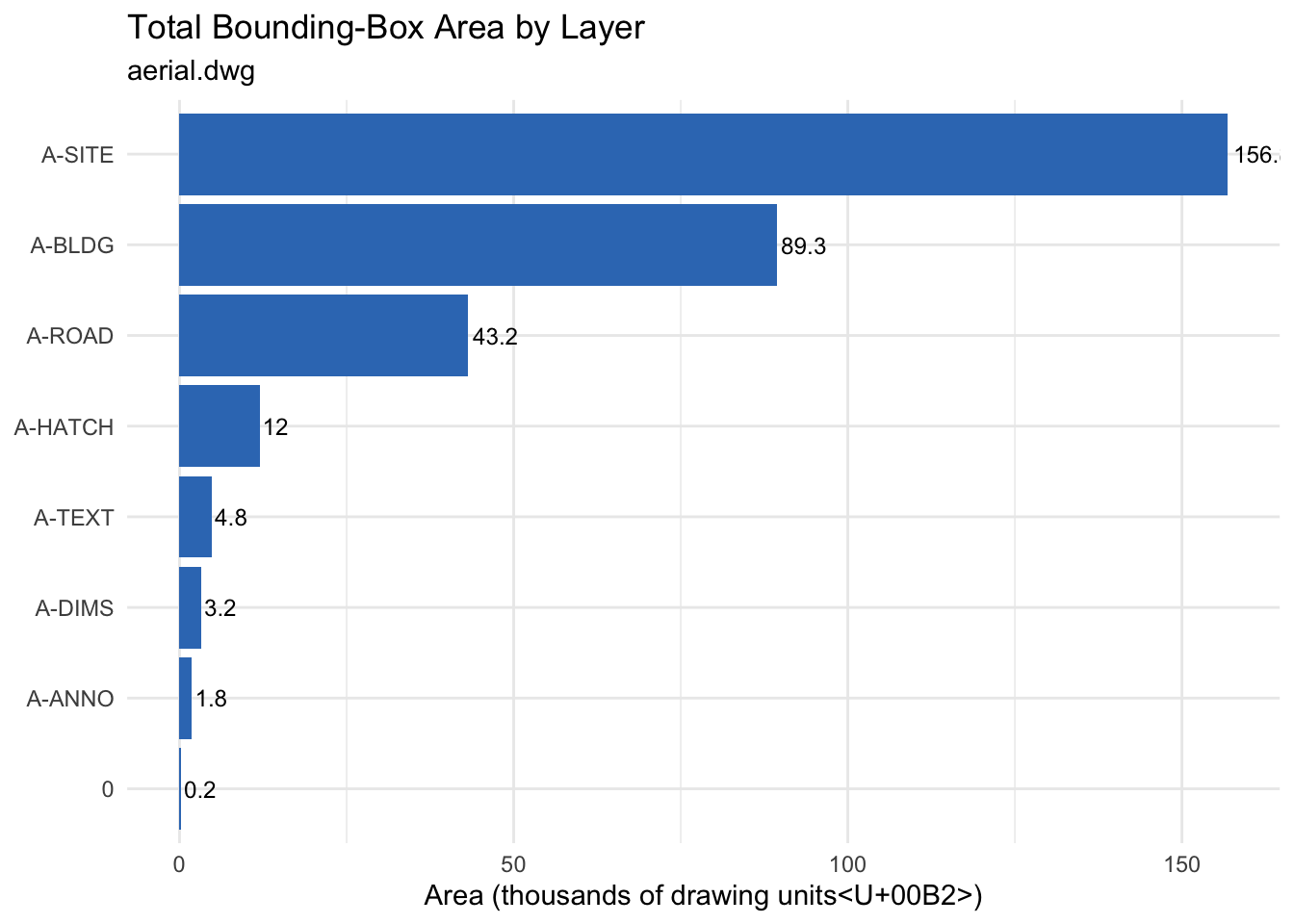

12.8 Objects per Layer — Dot Plot

A dot plot works better than a bar chart when you want to compare both count and area simultaneously:

ggplot(layer_summary, aes(x = n_objects, y = reorder(layer, n_objects))) +
  geom_point(aes(size = total_area / 1000), colour = "#367ABF", alpha = 0.8) +
  geom_text(aes(label = n_objects), hjust = -0.8, size = 3) +
  scale_size_continuous(name = "Total area\n(thousands of units²)",
                        range = c(2, 10)) +
  labs(title = "Objects per Layer",
       subtitle = "Point size proportional to total bounding-box area",
       x = "Object count", y = NULL) +
  theme_minimal()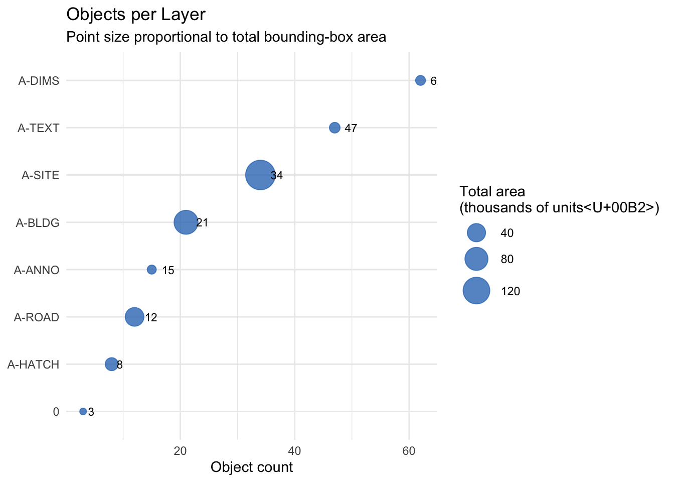

The props_df and layer_summary objects carry forward into Attribute Extraction and Cross-Drawing Comparison.