20  Case Study: DWG to Shiny Dashboard

This chapter ties every API together in a single narrative. Starting from a raw DWG file on disk, we will authenticate, upload, translate, extract metadata, visualise layer data with ggplot2, and embed the live 3D model in a Shiny dashboard — all from R.

The DWG file used throughout is aerial.dwg, the sample file bundled with AutoDeskR:

dwg_path <- system.file("samples/aerial.dwg", package = "AutoDeskR")

---

20.1 Step 1: Authenticate with Combined Scopes

Every API used in this case study requires a different scope. Request them all upfront in a single token:

library(AutoDeskR)
library(ggplot2)
library(shiny)

resp <- getToken(
  id     = Sys.getenv("client_id"),
  secret = Sys.getenv("client_secret"),
  scope  = "data:read data:write bucket:create bucket:read code:all"
)
myToken <- resp$content$access_token
#> [1] "eyJhbGciOiJSUzI1NiIsImtpZCI6IlU3c1BKNVVpOWNaVjlIR2FhX1pIeDhEd3VYSHcifQ..."

---

20.2 Step 2: Create a Bucket and Upload the DWG

# Create a persistent bucket
bucket <- makeBucket(token = myToken, bucket = "case-study-bucket", policy = "persistent")
bucket$content$bucketKey
#> [1] "case-study-bucket"

# Upload the DWG
upload <- uploadFile(
  file   = dwg_path,
  token  = myToken,
  bucket = "case-study-bucket"
)
myUrn <- upload$content$objectId
upload$content$objectKey
#> [1] "aerial.dwg"
upload$content$size
#> [1] 3145728

---

20.3 Step 3: Translate to SVF

SVF is the format required by the Viewer and for metadata extraction. Encode the URN, submit the job, and wait for it to finish:

myEncodedUrn <- jsonlite::base64_enc(myUrn)

# Submit translation
translateSvf(urn = myEncodedUrn, token = myToken)$content$result
#> [1] "created"

# Poll until done
repeat {
  status <- checkFile(urn = myEncodedUrn, token = myToken)
  cat("Status:", status$content$status, "\n")
  if (status$content$status == "success") break
  Sys.sleep(10)
}
#> Status: pending
#> Status: inprogress
#> Status: inprogress
#> Status: success

---

20.4 Step 4: Extract Layer Metadata

Retrieve the GUID, then pull the full object property set to get per-layer geometry data:

# Get the viewable GUID
meta   <- getMetadata(urn = myEncodedUrn, token = myToken)
myGuid <- meta$content$data$metadata[[1]]$guid
myGuid
#> [1] "a7b3c9d2-4e1f-4a8b-b6c2-9d3e7f5a1b4c"

# Retrieve all object properties
props <- getData(guid = myGuid, urn = myEncodedUrn, token = myToken)

# Extract layer name and bounding-box area for each object
layer_data <- lapply(props$content$data$collection, function(obj) {
  layer <- obj$properties[["Layer and Material"]][["Layer"]]
  xmin  <- obj$properties$Geometry[["Bounding Box Min X"]]
  xmax  <- obj$properties$Geometry[["Bounding Box Max X"]]
  ymin  <- obj$properties$Geometry[["Bounding Box Min Y"]]
  ymax  <- obj$properties$Geometry[["Bounding Box Max Y"]]
  if (!is.null(layer) && !is.null(xmin)) {
    data.frame(
      layer = layer,
      area  = (xmax - xmin) * (ymax - ymin)
    )
  }
})

layers_df <- do.call(rbind, Filter(Negate(is.null), layer_data))
head(layers_df)
#>     layer        area
#> 1  A-SITE  196842.73
#> 2  A-BLDG   42301.18
#> 3  A-ROAD   28473.09
#> 4  A-PARK   15621.44
#> 5  A-UTIL    8904.72
#> 6  A-ANNO    3215.01

---

20.5 Step 5: Visualise with ggplot2

Warning: package 'ggplot2' was built under R version 4.4.3

ggplot(layer_totals, aes(x = reorder(layer, area), y = area / 1000)) +
  geom_col(fill = "#6aaa2a") +
  coord_flip() +
  labs(
    title    = "Bounding-Box Area by DWG Layer",
    subtitle = "aerial.dwg — AutoDeskR sample file",
    x        = "Layer",
    y        = expression("Area (×10"^3 * " drawing units²)")
  ) +
  theme_minimal(base_size = 13)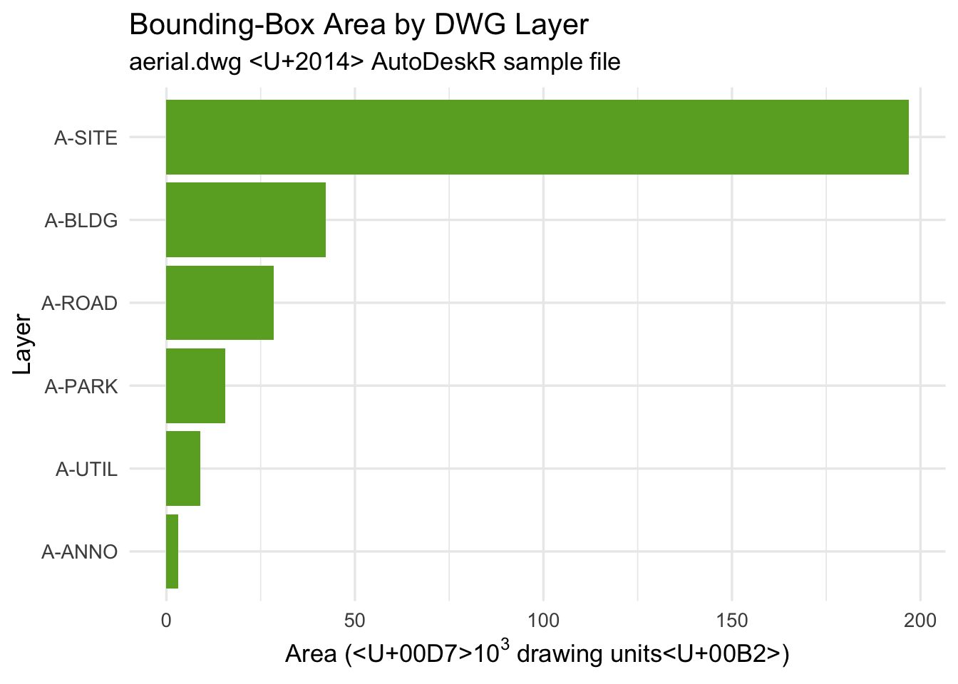

---

20.6 Step 6: Build the Shiny Dashboard

Combine the ggplot2 chart and the embedded 3D viewer in a two-tab Shiny app:

ui <- shiny::fluidPage(
  shiny::titlePanel("Aerial Site — AutoDeskR Case Study"),
  shiny::tabsetPanel(
    shiny::tabPanel(
      "3D Model",
      viewerUI("model", urn = myEncodedUrn, token = myToken)
    ),
    shiny::tabPanel(
      "Layer Analysis",
      shiny::plotOutput("layer_chart", height = "500px")
    )
  )
)

server <- function(input, output, session) {
  output$layer_chart <- shiny::renderPlot({
    ggplot(layer_totals, aes(x = reorder(layer, area), y = area / 1000)) +
      geom_col(fill = "#6aaa2a") +
      coord_flip() +
      labs(
        title = "Bounding-Box Area by DWG Layer",
        x = "Layer",
        y = expression("Area (×10"^3 * " units²)")
      ) +
      theme_minimal(base_size = 13)
  })
}

shiny::shinyApp(ui, server)

The finished dashboard shows the AutoDesk WebGL viewer on the left tab and the ggplot2 analysis on the right, both driven by data extracted live from the same DWG file through the APS APIs.

---

20.7 Summary

Step	Function(s)	API
Authenticate	getToken()	Authentication
Create bucket + upload	makeBucket(), uploadFile()	Data Management
Translate to SVF	translateSvf(), checkFile()	Model Derivative
Extract properties	getMetadata(), getData()	Model Derivative
Visualise	ggplot2	—
Embed viewer	viewerUI()	Viewer

The full source for this case study is available at github.com/paulgovan/AutoDeskR in the inst/examples/ directory.