library(dplyr)

std_cats <- c("Layer and Material", "Geometry", "General")

custom_df <- lapply(collection, function(obj) {
  props_flat  <- unlist(obj$properties, use.names = TRUE)
  custom_keys <- names(props_flat)[
    !grepl(paste(std_cats, collapse = "|"), names(props_flat))
  ]
  if (length(custom_keys) == 0) return(NULL)
  data.frame(objectid   = obj$objectid,
             prop_name  = custom_keys,
             prop_value = props_flat[custom_keys],
             stringsAsFactors = FALSE)
}) |> do.call(what = rbind)

head(custom_df)
#>   objectid              prop_name      prop_value
#> 1       42        Custom.Zone          Zone A
#> 2       42 Custom.Construction.Type   RC Frame
#> 3       42     Custom.Floor.Area          428.5
#> 4 43 Custom.Zone Zone B13 Attribute Extraction
Layer names and bounding boxes are just the start. DWG files also carry custom properties and block attributes, zone designations, construction types, sheet numbers, column marks, that make the drawing data genuinely useful for analysis. This chapter extracts those properties from the getData() response and reshapes them into analysis-ready data frames.
This chapter uses collection from Layer Structure Analysis.
13.1 Custom Properties
Custom properties appear under non-standard category names in obj$properties. The standard categories to exclude are "Layer and Material", "Geometry", and "General":
13.2 Block Attributes
Block inserts carry named attributes, found under the obj$properties$Attributes element:
block_df <- lapply(collection, function(obj) {
  if (is.null(obj$properties$Attributes)) return(NULL)
  attrs <- obj$properties$Attributes
  data.frame(objectid   = obj$objectid,
             block_name = obj$name,
             attr_name  = names(attrs),
             attr_value = unlist(attrs),
             stringsAsFactors = FALSE)
}) |> do.call(what = rbind)

head(block_df)
#>   objectid  block_name    attr_name  attr_value
#> 1       88 TITLE-BLOCK   SHEET_NO      A-001
#> 2       88 TITLE-BLOCK   REVISION      Rev 3
#> 3       89  COLUMN-TAG   MARK          C1
#> 4       89  COLUMN-TAG   GRID          A/1
13.3 Pivot to Wide Format
Long-form property data is easy to filter but awkward to join. pivot_wider() gives you one column per property:
library(tidyr)

custom_wide <- custom_df |>
  mutate(prop_name = sub("^Custom\\.", "", prop_name)) |>
  pivot_wider(names_from  = prop_name,
              values_from = prop_value)

head(custom_wide)
#> # A tibble: 3 × 4
#>   objectid Zone   Construction.Type Floor.Area
#>      <int> <chr>  <chr>             <chr>
#> 1       42 Zone A RC Frame          428.5
#> 2       43 Zone B Steel Frame       312.0
#> 3       51 Zone A Masonry           198.3
13.4 Join Attributes to Layer Data
Merge custom properties back onto the geometry data frame for combined analysis:
enriched <- props_df |>
  left_join(custom_wide, by = "objectid")
13.5 Floor Area by Zone and Construction Type
zone_summary <- enriched |>
  filter(layer == "A-BLDG", !is.na(Zone)) |>
  mutate(floor_area = as.numeric(Floor.Area)) |>
  group_by(Zone, Construction.Type) |>
  summarise(total_floor_area = sum(floor_area, na.rm = TRUE),
            n_units          = n(),
            .groups          = "drop")

zone_summary
#> # A tibble: 3 × 4
#>   Zone   Construction.Type total_floor_area n_units
#> 1 Zone A Masonry                      198.3       1
#> 2 Zone A RC Frame                     428.5       1
#> 3 Zone B Steel Frame                  312.0       1
13.6 Visualising Custom Attributes
A stacked bar chart of floor area by zone and construction type:
ggplot(zone_summary,
       aes(x = Zone, y = total_floor_area, fill = Construction.Type)) +
  geom_col(position = "stack") +
  geom_text(aes(label = paste0(round(total_floor_area, 0), " m²")),
            position = position_stack(vjust = 0.5),
            colour = "white", size = 3.5) +
  scale_fill_manual(values = c("#367ABF", "#4CAF50", "#F4A261")) +
  labs(title = "Floor Area by Zone and Construction Type",
       subtitle = "Extracted from block attributes — aerial.dwg",
       x = NULL, y = "Floor area (m²)", fill = "Construction type") +
  theme_minimal()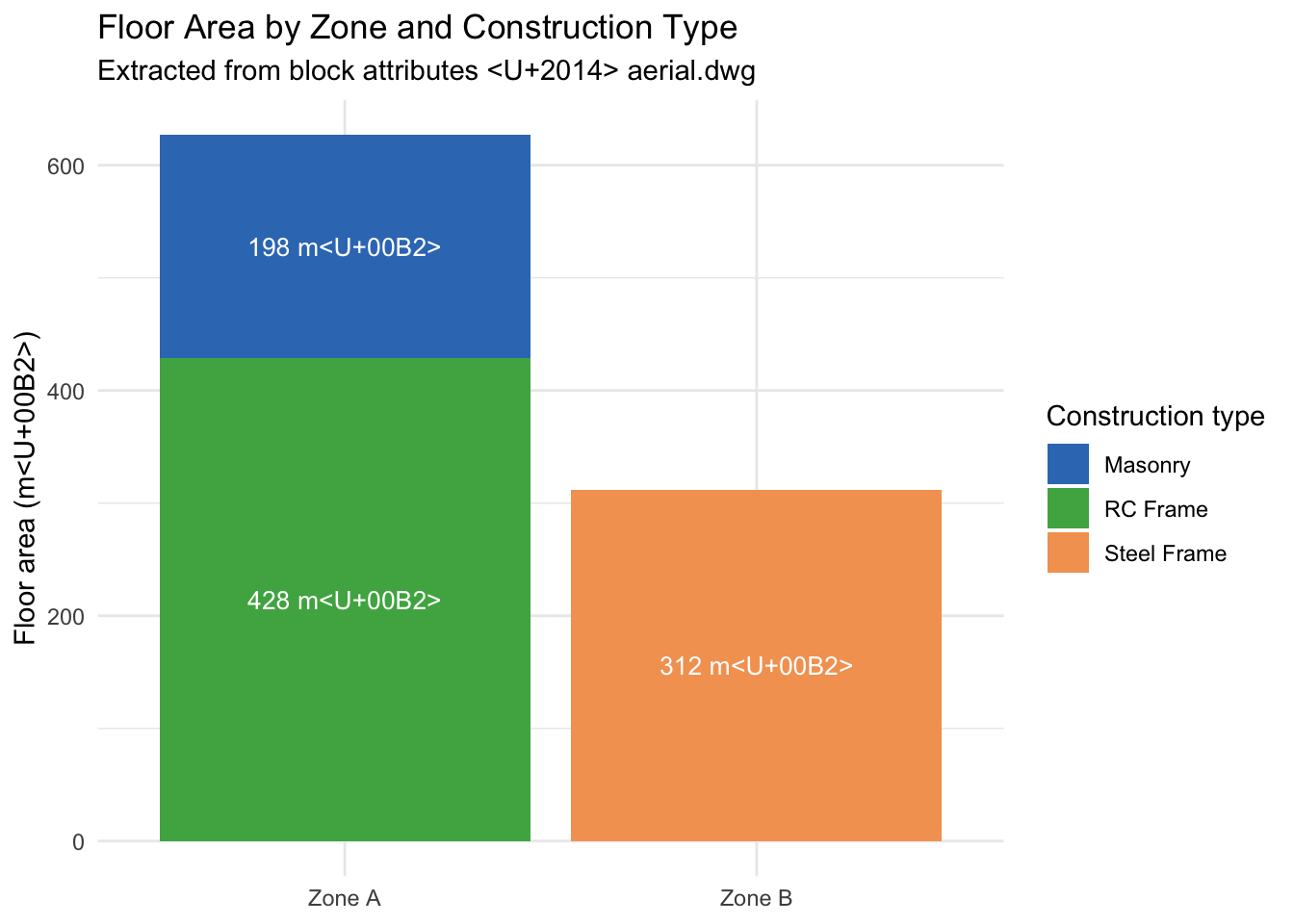
13.7 Export
Write the enriched data frame to CSV for handover or further processing:
write.csv(enriched, file = "drawing_attributes.csv", row.names = FALSE)