8 Mesh Metrics

Got a mesh? Let’s measure it. Rvcg (Schlager 2024) and geometry (Roussel, Sterratt, et al. 2024) turn a tmesh3d into a full geometric report, surface area, volume, bounding box, centroid. These numbers are useful for QA (does the translated geometry match the design intent?), quantity takeoff, and as inputs to dashboards and reports.

This chapter uses mesh_vcg from Reading OBJ and STL Meshes.

8.1 Surface Area

library(Rvcg)
area <- vcgArea(mesh_vcg)
area
#> [1] 14823.6   # square units — same as the DWG drawing units

8.2 Volume

vol <- vcgVolume(mesh_vcg)
vol
#> [1] 48219.3

Warning

vcgVolume() only gives meaningful results for watertight (closed) meshes. OBJ files translated from open 2D DWG drawings are almost never watertight, so this number will be unreliable. Use the convex hull fallback below instead.

8.3 Bounding Box

bb <- apply(t(mesh_vcg$vb[1:3, ]), 2, range)
rownames(bb) <- c("min", "max")
colnames(bb) <- c("X", "Y", "Z")
bb
#>        X        Y      Z
#> min -142.83  -98.47   0.00
#> max  318.62  241.19  12.50

diff(bb)   # width / depth / height
#>       X      Y     Z
#> 461.45 339.66 12.50

8.4 Centroid

centroid <- colMeans(t(mesh_vcg$vb[1:3, ]))
names(centroid) <- c("X", "Y", "Z")
centroid
#>      X      Y     Z
#>  87.90  71.36   6.25

8.5 Convex Hull Volume

For open (non-watertight) meshes, geometry::convhulln() (Roussel, Sterratt, et al. 2024) computes the volume and surface area of the convex hull, a conservative upper bound that doesn’t require a closed surface:

library(geometry)
pts  <- t(mesh_vcg$vb[1:3, ])
hull <- convhulln(pts, options = "FA")
hull$vol
#> [1] 1871423.5
hull$area
#> [1] 216834.2

8.6 Summary Table

Pull all the numbers together into a single data frame, ready to feed into a gt table or write to CSV:

mesh_summary <- data.frame(
  metric = c("Vertices", "Faces", "Surface area",
             "Convex hull volume", "Convex hull area",
             "Bounding box X", "Bounding box Y", "Bounding box Z",
             "Centroid X", "Centroid Y", "Centroid Z"),
  value  = c(ncol(mesh_vcg$vb), ncol(mesh_vcg$it), area,
             hull$vol, hull$area,
             diff(bb)[1], diff(bb)[2], diff(bb)[3],
             centroid[1], centroid[2], centroid[3])
)
mesh_summary
#>                metric        value
#> 1            Vertices     2847.000
#> 2               Faces     1832.000
#> 3        Surface area    14823.600
#> 4  Convex hull volume  1871423.500
#> 5    Convex hull area   216834.200
#> 6      Bounding box X      461.450
#> 7      Bounding box Y      339.660
#> 8      Bounding box Z       12.500
#> 9          Centroid X       87.900
#> 10         Centroid Y       71.360
#> 11         Centroid Z        6.250

8.7 Visualising the Metrics

A quick bar chart makes the bounding box dimensions easy to compare at a glance:

Warning: package 'ggplot2' was built under R version 4.4.3

ggplot(bbox_df, aes(x = dimension, y = value, fill = dimension)) +
  geom_col(show.legend = FALSE) +
  geom_text(aes(label = round(value, 1)), vjust = -0.4, size = 3.5) +
  scale_fill_manual(values = c("#367ABF", "#4CAF50", "#F4A261")) +
  labs(title = "Bounding Box Dimensions",
       subtitle = "aerial.dwg — translated mesh",
       x = NULL, y = "Drawing units") +
  theme_minimal()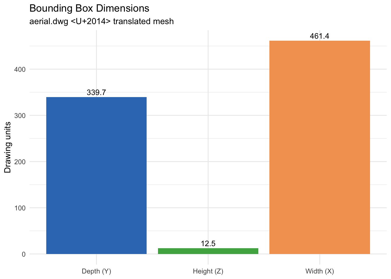

These metrics can be passed to a gt table for a polished handover report. See Automated Drawing Reports for the formatting details.