Introduction
Welcome to PRA! This project provides a set of tools for performing Project Risk Analysis (PRA) using various quantitative methods. It is designed to help project analysts assess and manage risks associated with project schedules, costs, and performance.
PRA can be used as a traditional R package with direct function calls, or driven by AI agents: every analytical function is exposed as a tool over the Model Context Protocol (MCP), and the package ships a set of Agent Skills that tell an agent when and how to call each tool.
Key Features
AI Agent Integration
-
MCP server —
pra_mcp_server()exposes every analytical function as a tool over the Model Context Protocol, callable from Claude, Claude Code, and other MCP-compatible clients -
Agent Skills — bundled
SKILL.mdfiles (undersystem.file("skills", package = "PRA")) document when to use each method, which tool to call, the JSON argument format, and how to interpret results -
No embedded model — all analytical functions run without any AI dependency; only the MCP server needs the optional
ellmer,mcptools, andjsonlitepackages
See the Agentic Risk Analysis chapter for details.
Installation
To install the release version of PRA, use:
install.packages('PRA')You can install the development version of PRA like so:
devtools::install_github('paulgovan/PRA')Usage
Traditional R Interface
Here is a simple example of how to use the package for a common PRA task.
First, load the package:
Suppose you have a simple project with 3 tasks (A, B, and C), but the duration of each task is uncertain. You can describe the uncertainty of each task using probability distributions and then run a Monte Carlo Simulation (MCS) to estimate the overall project duration.
To do so, set the number of simulations and describe probability distributions for each work package. In this case, run 10,000 simulations with the following distributions:
num_simulations <- 10000
task_distributions <- list(
  list(type = "normal", mean = 10, sd = 2), # Task A: Normal distribution
  list(type = "triangular", a = 5, b = 10, c = 15), # Task B: Triangular distribution
  list(type = "uniform", min = 8, max = 12) # Task C: Uniform distribution
)
Then run the simulation using the mcs function and store the results:
results <- mcs(num_simulations, task_distributions)To visualize the results, you can create a histogram of the total project duration. You can also overlay a normal distribution curve based on the mean and standard deviation of the results:
hist(results$total_distribution,
  freq = FALSE, breaks = 50, main = "Distribution of Total Project Duration",
  xlab = "Total Duration", col = "skyblue", border = "white"
)
curve(dnorm(x, mean = results$total_mean, sd = results$total_sd), add = TRUE, col = "darkblue")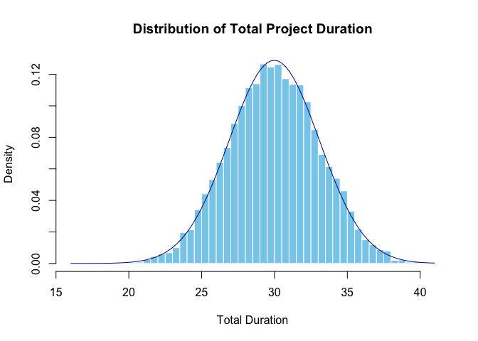
This will give you a visual representation of the uncertainty in the total project duration based on the individual task distributions. On average, the project is expected to take around 30 time units, but could take as little as 20 or as much as 40 time units.
AI Agent Interface
PRA exposes all of its analytical functions to AI agents through an MCP server. Start it from an R session, or register it with an MCP-compatible client.
Register with Claude Code:
Register with Claude Desktop (add to the MCP configuration file):
Once connected, the agent can call tools such as mcs_tool, evm_analysis_tool, risk_prob_tool, and grandparent_dsm_tool as native tools. The bundled Agent Skills guide the agent on when and how to use each one:
# Locate the installed skill files
list.files(system.file("skills", package = "PRA"))
More Resources
This project was inspired by the book Data Analysis for Engineering and Project Risk Managment by Ivan Damnjanovic and Ken Reinschmidt and is highly recommended.
Code of Conduct
Please note that the PRA project is released with a Contributor Code of Conduct. By contributing to this project, you agree to abide by its terms.