This function performs a Monte Carlo simulation to estimate the total duration of a project based on individual task distributions and an optional correlation matrix.
Arguments
- num_sims
The number of simulations to run.
- task_dists
A list of lists describing each task distribution with its parameters. Each task distribution should be specified as a list with a "type" field (indicating the distribution type: "normal", "triangular", or "uniform") and the corresponding parameters: for "normal" (mean, sd), for "triangular" (a, b, c), and for "uniform" (min, max). For example: list( list(type = "normal", mean = 10, sd = 2), list(type = "triangular", a = 5, b = 10, c = 15), list(type = "uniform", min = 8, max = 12) )
- cor_mat
The correlation matrix for the tasks (Optional). If not provided, tasks are assumed to be independent.
Value
An S3 object of class "mcs": a list of the total mean, variance,
standard deviation, percentiles, and the simulated total distribution.
Objects of this class have print.mcs(), summary.mcs() and plot.mcs()
methods.
Note
When a correlation matrix is supplied, dependence is induced by
Cholesky decomposition. The correlation matrix is factored, independent
standard normal scores are multiplied by the Cholesky factor to carry the
target correlation, and each column is then returned to its own scale through
the normal CDF and that task's inverse CDF. Applying the factor to standard
normal scores rather than to the raw task draws is required for the
factorization to be valid, since it presumes unit-variance inputs. Every
marginal distribution is therefore preserved exactly. The sampled rank
correlation matches the target matrix, while the product-moment correlation
is approximate: it is attenuated for strongly skewed marginals, an inherent
property of the transform. smm() remains available when only first and second moments are
needed; see the package's design-structure tools for modeling structural
dependence directly.
References
Damnjanovic, Ivan, and Kenneth Reinschmidt. Data analytics for engineering and construction project risk management. No. 172534. Cham, Switzerland: Springer, 2020.
Examples
# Set the number of simulations and task distributions for a toy project.
num_sims <- 10000
task_dists <- list(
  list(type = "normal", mean = 10, sd = 2), # Task A: Normal distribution
  list(type = "triangular", a = 5, b = 10, c = 15), # Task B: Triangular distribution
  list(type = "uniform", min = 8, max = 12) # Task C: Uniform distribution
)

# Set the correlation matrix for the correlations between tasks.
cor_mat <- matrix(c(
  1, 0.5, 0.3,
  0.5, 1, 0.4,
  0.3, 0.4, 1
), nrow = 3, byrow = TRUE)

# Run the Monte Carlo sumulation and print the results.
results <- mcs(num_sims, task_dists, cor_mat)
cat("Mean Total Duration:", results$total_mean, "\n")
#> Mean Total Duration: 30.03153
cat("Variance of Total Variance:", results$total_variance, "\n")
#> Variance of Total Variance: 16.95771
cat("Standard Deviation of Total Duration:", results$total_sd, "\n")
#> Standard Deviation of Total Duration: 4.117973
cat("5th Percentile:", results$percentiles[1], "\n")
#> 5th Percentile: 23.25509
cat("Median (50th Percentile):", results$percentiles[2], "\n")
#> Median (50th Percentile): 29.9976
cat("95th Percentile:", results$percentiles[3], "\n")
#> 95th Percentile: 36.80591
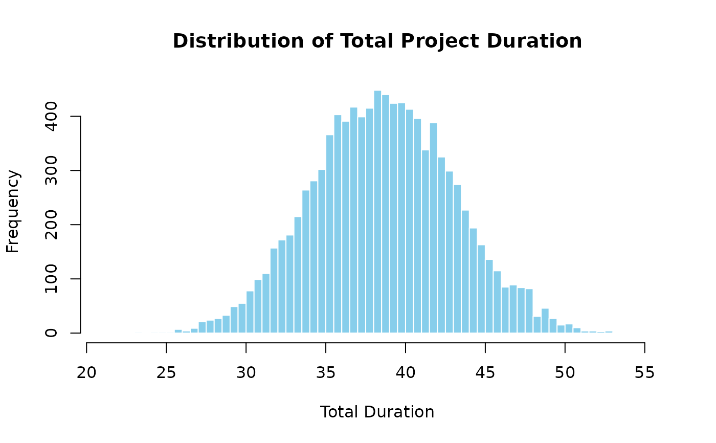
hist(results$total_distribution,
  breaks = 50, main = "Distribution of Total Project Duration",
  xlab = "Total Duration", col = "skyblue", border = "white"
)
legend("topright", legend = c("Total Duration Distribution"), fill = c("skyblue"))