8  Web-Based Analysis with ReliaShiny

8.1 Introduction

All of the analyses in this book require writing R code. ReliaShiny (Govan 2023) removes that requirement — it is a point-and-click Shiny (Chang et al. 2022) web application that exposes the same reliability analysis workflows (RAM, life data analysis, reliability testing, repairable systems, reliability block diagrams) through a graphical interface. No R programming knowledge is needed to run an analysis.

This chapter introduces ReliaShiny, tours its modules, and explains when to reach for it versus a scripted R workflow.

8.2 Installation and Launch

ReliaShiny is available on CRAN:

install.packages("ReliaShiny")

Once installed, launch the app from the R console:

library(ReliaShiny)
ReliaShiny()

This opens the application in your default web browser. The app runs locally — no internet connection or account is required.

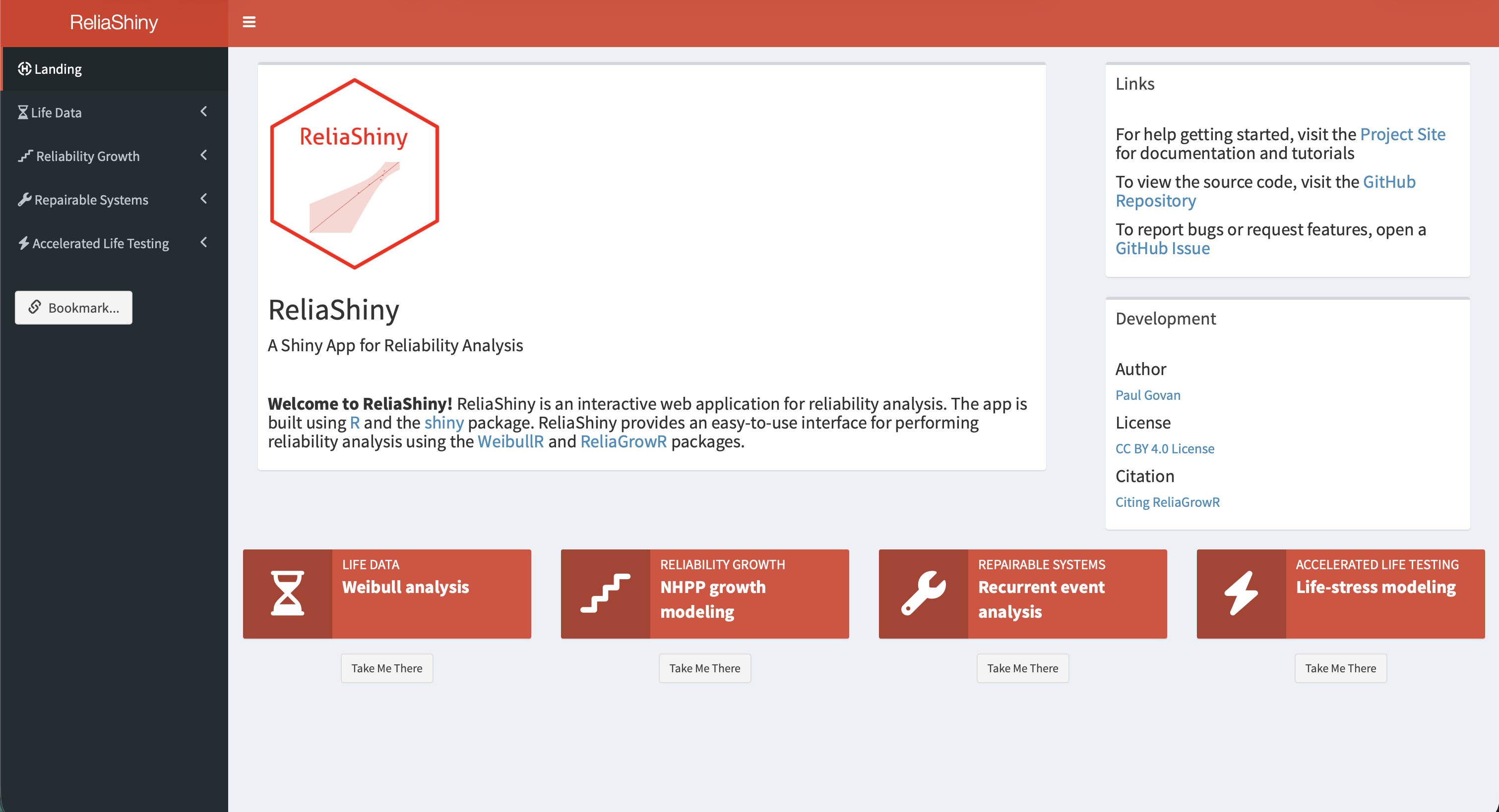
8.3 App Overview

When ReliaShiny opens, the left sidebar displays the available analysis modules, each corresponding to a chapter in this book:

ReliaShiny landing page showing the sidebar module list.

Module	Corresponding chapter	Key capabilities
RAM	Chapter 1	Reliability, availability, MTTF, MTBF, failure rate
Life Data Analysis	Chapter 3	2-parameter, 3-parameter Weibull, Weibayes; MRR and MLE; right-censored data
Reliability Growth	Chapter 4	Duane and Crow-AMSAA model fitting; piecewise NHPP
Accelerated Life Testing	Chapter 5	Arrhenius and Power Law models; relationship plots
Repairable Systems	Chapter 6	Power Law Process (NHPP); MCF; fleet exposure
Reliability Block Diagrams	Chapter 2	Series, parallel, mixed, and k-out-of-n configurations

Each module follows the same three-step workflow:

1. Input — enter or upload your data using form fields, tables, or file uploads.
2. Analyze — click Run to fit the model.
3. Output — view plots, parameter estimates, and summary statistics; download results.

8.4 Module Walkthroughs

RAM Module

The RAM module computes reliability, availability, MTTR, MTTF, MTBF, and failure rate from summary inputs.

Workflow:

1. Select the RAM tab in the sidebar.
2. Enter the total time, failed time, and (for availability) scheduled maintenance time.
3. Click Calculate.
4. The panel displays all five metrics: Reliability, Availability, MTTR, MTTF, MTBF, and Failure Rate.

This mirrors the rel(), avail(), mttf(), mtbf(), and fr() helper functions from Chapter 1.

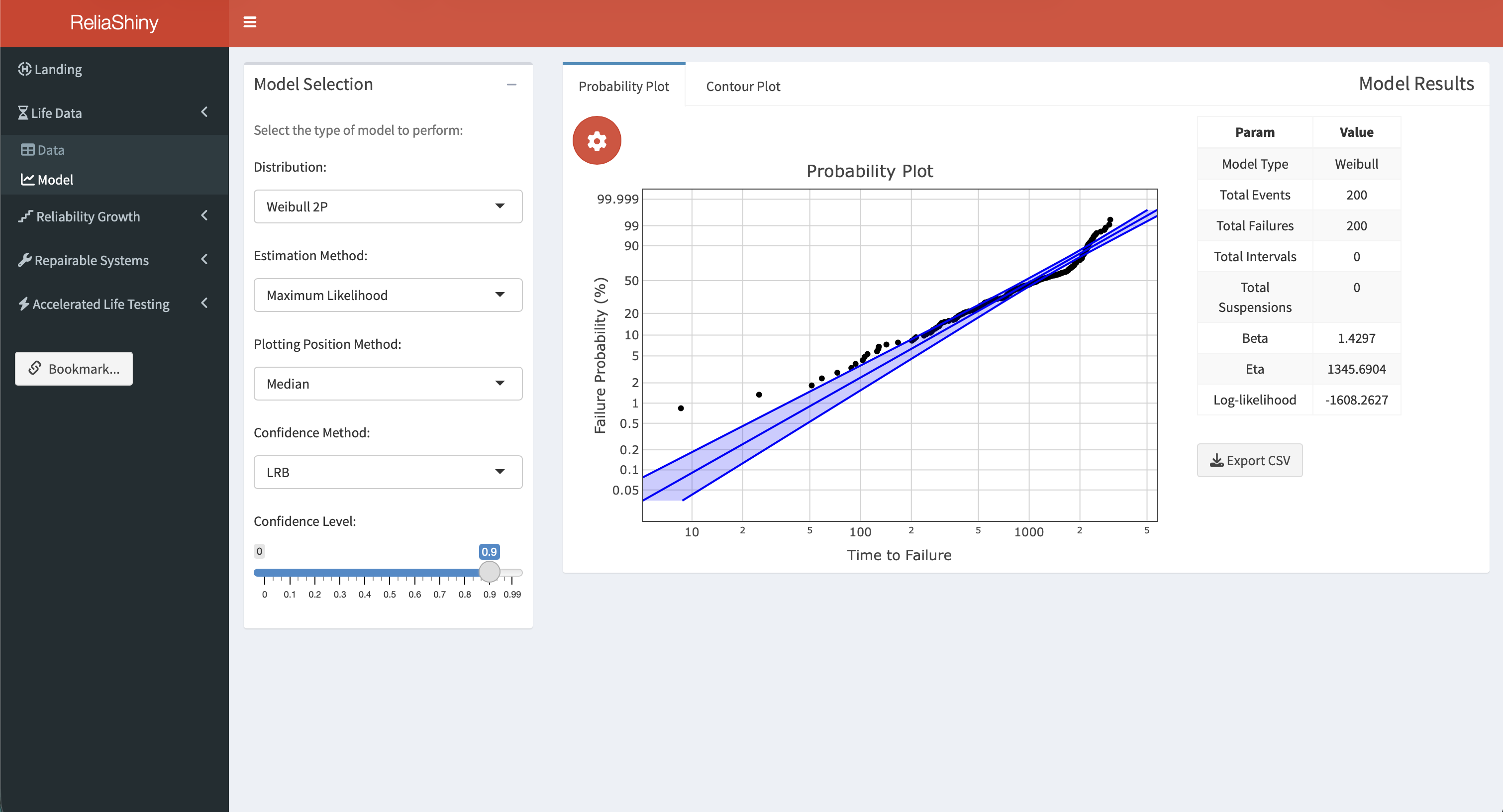
Life Data Analysis Module

The LDA module fits Weibull models and generates probability plots.

LDA module showing a fitted Weibull probability plot.

Workflow:

1. Select the Life Data Analysis tab.
2. Upload data — paste failure times into the input table, or upload a CSV with columns time and event (1 = failure, 0 = suspension).
3. Choose model — 2-parameter Weibull (default), 3-parameter Weibull, or Weibayes.
4. Choose estimation method — MRR or MLE.
5. Click Fit Model.
6. The probability plot appears in the main panel, with \(\hat{\beta}\), \(\hat{\eta}\), and the Anderson-Darling statistic in the sidebar.
7. Click Download Plot to save the chart as a PNG.

CSV format for upload:

time,event
30,1
49,1
82,1
90,1
96,1
100,0
45,0
10,0

A 0 in the event column marks a suspension (right-censored observation).

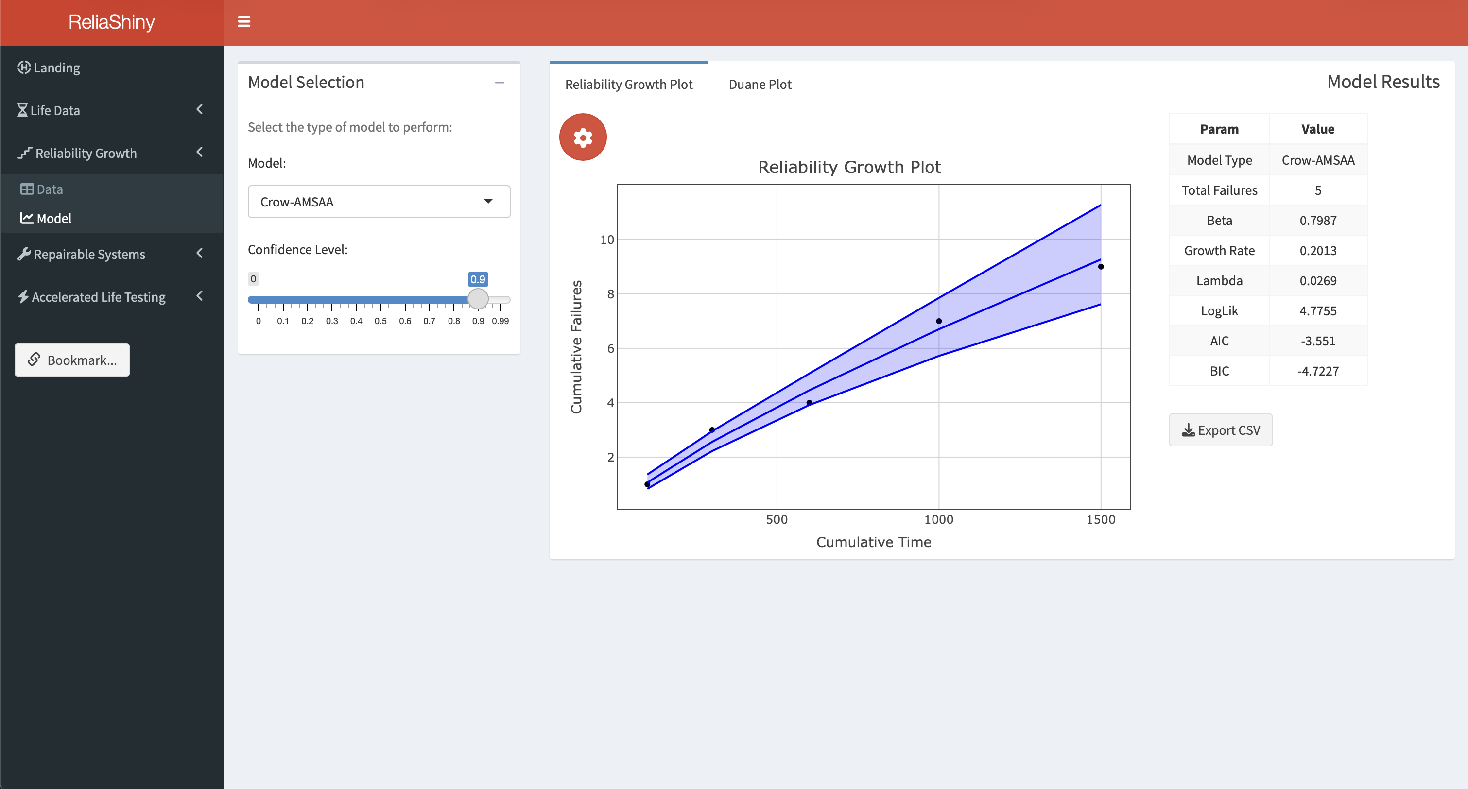
Reliability Growth Module

The Reliability Growth module fits Duane and Crow-AMSAA reliability growth models.

Reliability Growth module showing a fitted Crow-AMSAA cumulative failures plot.

Workflow:

1. Select Reliability Growth.
2. Enter cumulative test times and failure counts in the data table.
3. Choose Duane or Crow-AMSAA model.
4. Click Fit.
5. The plot shows the fitted model; \(\hat{\beta}\) and model parameters appear in the results panel.

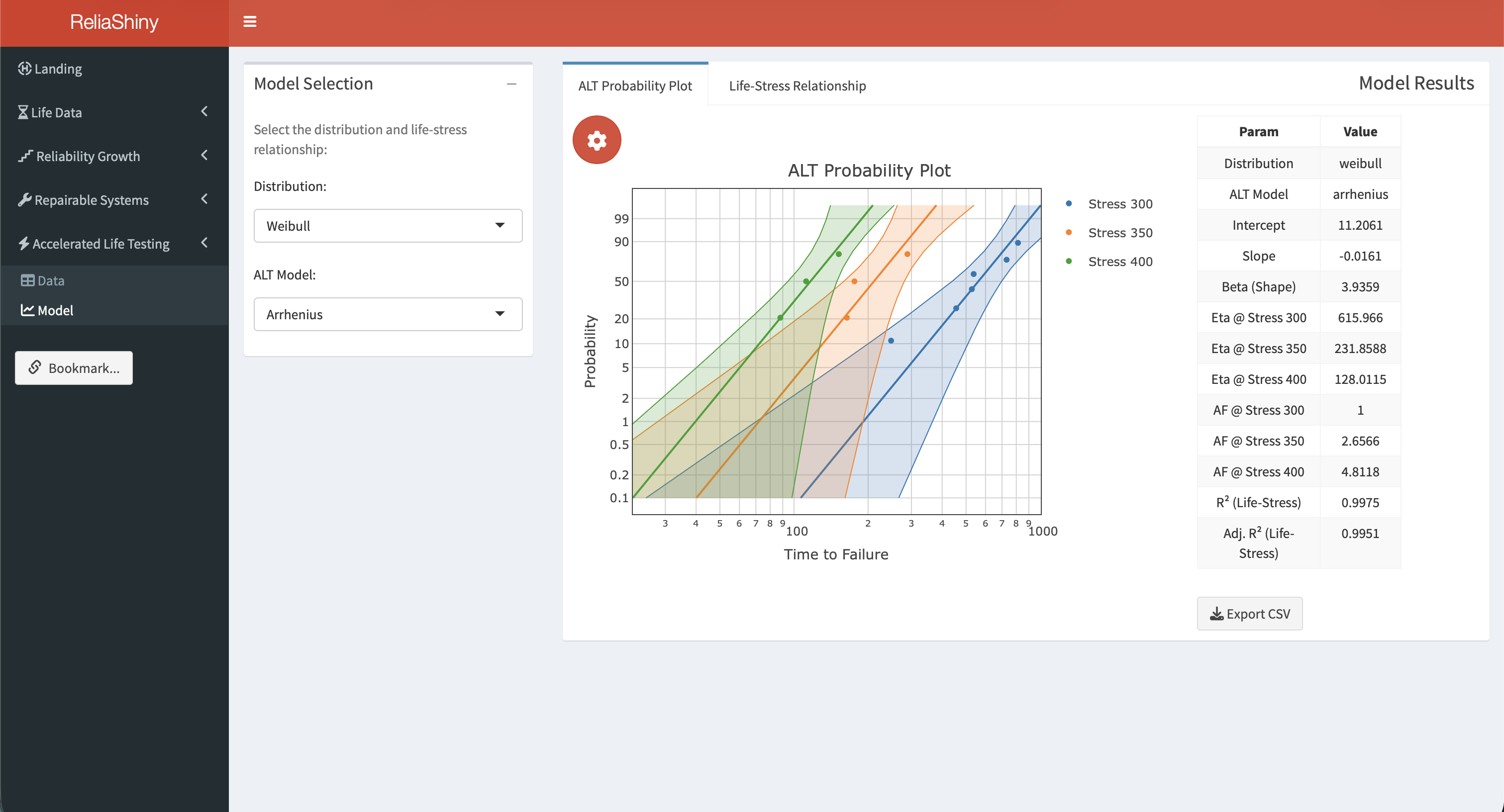
Accelerated Life Testing Module

The ALT module fits Arrhenius and Power Law acceleration models using the WeibullR.ALT package (see Chapter 5).

ALT module showing a probability plot and life-stress relationship.

Workflow:

1. Select Accelerated Life Testing.
2. Upload a dataset with columns time, event, qty, and a stress column (e.g., TempC or Voltage).
3. Choose the acceleration model: Arrhenius (temperature) or Power Law (mechanical/voltage stress).
4. Click Fit ALT Model.
5. The probability plot and relationship plot are displayed, along with fitted parameters and the computed Acceleration Factor.

Repairable Systems Module

The Repairable Systems module fits the Power Law Process (Crow-AMSAA) and computes the MCF for fleet data.

Repairable Systems module showing a Mean Cumulative Function plot.

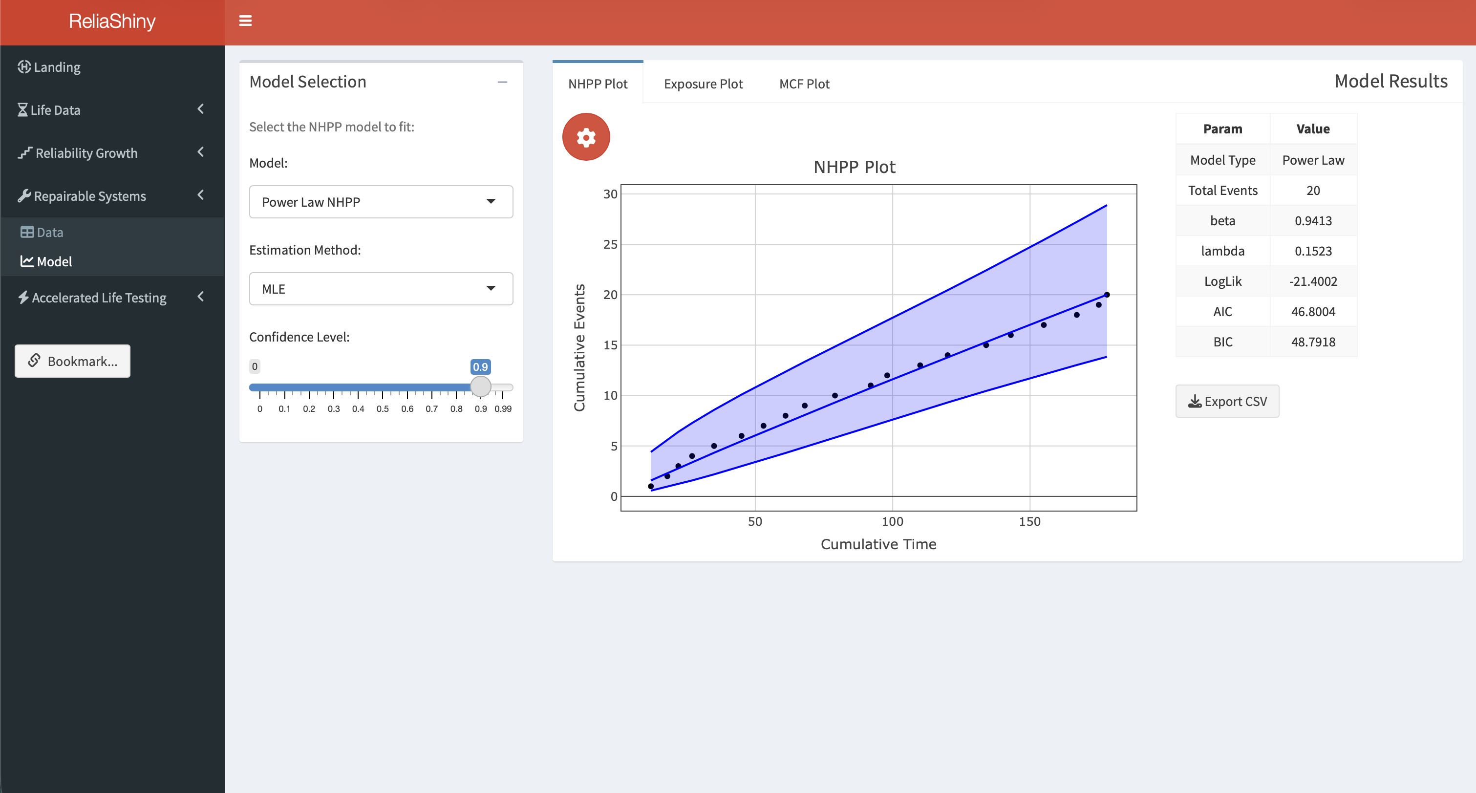
Workflow:

1. Select Repairable Systems.
2. Upload fleet data with columns id, time, and event.
3. Choose analysis type: NHPP (Power Law) or MCF.
4. Optionally enter a breakpoint for piecewise NHPP fitting.
5. Click Analyze.
6. The cumulative failures plot (NHPP) or MCF curve is displayed, with estimated parameters.

Example CSV format:

id,time,event
1,310,1
1,850,1
1,1620,1
2,420,1
2,1050,1
2,3000,0

The last row for system 2 (event = 0) indicates that system 2 was observed until hour 3,000 without a third failure.

Reliability Block Diagrams Module

The RBD module computes system reliability from component reliabilities for series, parallel, mixed, and k-out-of-n configurations.

Workflow:

1. Select Reliability Block Diagrams.
2. Choose the system topology from the dropdown: Series, Parallel, Mixed, or k-out-of-n.
3. Enter the number of components and their individual reliabilities.
4. For Mixed systems, define subsystem groupings.
5. For k-out-of-n systems, enter \(k\) (minimum required) and \(n\) (total).
6. Click Calculate.
7. System reliability and, for exponential components, system MTTF are displayed.
8. A block diagram graphic is shown for Series and Parallel configurations.

8.5 Data Upload Tips

• CSV files: core column names (time, event, id, qty) are case-sensitive and must be lowercase. Stress column names (e.g., TempC, Voltage) may use any valid R name — they are selected in the app’s dropdown.
• Missing values: rows with NA in the time column are automatically excluded.
• Large datasets: the app handles datasets up to ~10,000 rows without performance issues.
• Units: ReliaShiny is unit-agnostic — use hours, years, cycles, or any consistent unit. Label your outputs accordingly.

8.6 Downloading Results

Every module provides download buttons for:

• Plot PNG — the current chart at screen resolution.
• Results CSV — parameter estimates and summary statistics in tabular form.
• Report HTML — a self-contained report combining the inputs, plot, and results (available in LDA and RT modules).

8.7 When to Use ReliaShiny vs Scripted R

Situation	ReliaShiny	Scripted R
Quick one-off analysis	✅
Teaching / demonstration	✅
Sharing with non-R users	✅
Automating repeated analyses		✅
Custom plots and formatting		✅
Reproducible research / version control		✅
Embedding results in a Quarto book		✅
Large batch processing		✅

ReliaShiny excels at rapid exploration, prototyping, and sharing results with stakeholders who do not use R. For production workflows, automated pipelines, and fully reproducible analyses, scripted R with the underlying packages (WeibullR, ReliaGrowR, WeibullR.ALT) gives more control.

8.8 Getting Help

Within the app, click the ? icon on any panel for a tooltip explaining the inputs and outputs for that module.

From R:

help(package = "ReliaShiny")

Additional resources:

• CRAN page: https://CRAN.R-project.org/package=ReliaShiny

8.9 Summary

ReliaShiny provides a point-and-click interface to the full ReliaLearnR analysis ecosystem — RAM, life data analysis, reliability testing, repairable systems, and reliability block diagrams — with no R coding required. Install it with install.packages("ReliaShiny") and launch it with ReliaShiny(). Use it for rapid exploration, stakeholder demonstrations, and sharing results; switch to scripted R for reproducibility, automation, and custom outputs.

Chang, Winston, Joe Cheng, JJ Allaire, et al. 2022. Shiny: Web Application Framework for r. https://doi.org/10.32614/CRAN.package.shiny.

Govan, Paul. 2023. ReliaShiny: A ’Shiny’ App for Reliability Analysis. https://doi.org/10.32614/CRAN.package.ReliaShiny.