Contingency Calculation.

This function calculates the contingency required for a project based on the results of a Monte Carlo simulation. The contingency is determined by the difference between the specified high percentile (phigh) and the base percentile (pbase) of the total project duration distribution.

Usage

contingency(sims, phigh = 0.95, pbase = 0.5)

Arguments

sims

List of results from a Monte Carlo simulation containing the total project duration distribution.

phigh

Percentile level for contingency calculation. Default is 0.95 (95th percentile).

pbase

Base level for contingency calculation. Default is 0.5 (50th percentile).

Value

The function returns the value of calculated contingency based on the specified percentiles.

Examples

# Set the number os simulations and the task distributions for a toy project.
num_sims <- 10000
task_dists <- list(
  list(type = "normal", mean = 10, sd = 2), # Task A: Normal distribution
  list(type = "triangular", a = 5, b = 10, c = 15), # Task B: Triangular distribution
  list(type = "uniform", min = 8, max = 12) # Task C: Uniform distribution
)

# Set the correlation matrix for the correlations between tasks.
cor_mat <- matrix(c(
  1, 0.5, 0.3,
  0.5, 1, 0.4,
  0.3, 0.4, 1
), nrow = 3, byrow = TRUE)

# Run the Monte Carlo simulation.
results <- mcs(num_sims, task_dists, cor_mat)

# Calculate the contingency and print the results.
contingency <- contingency(results, phigh = 0.95, pbase = 0.50)
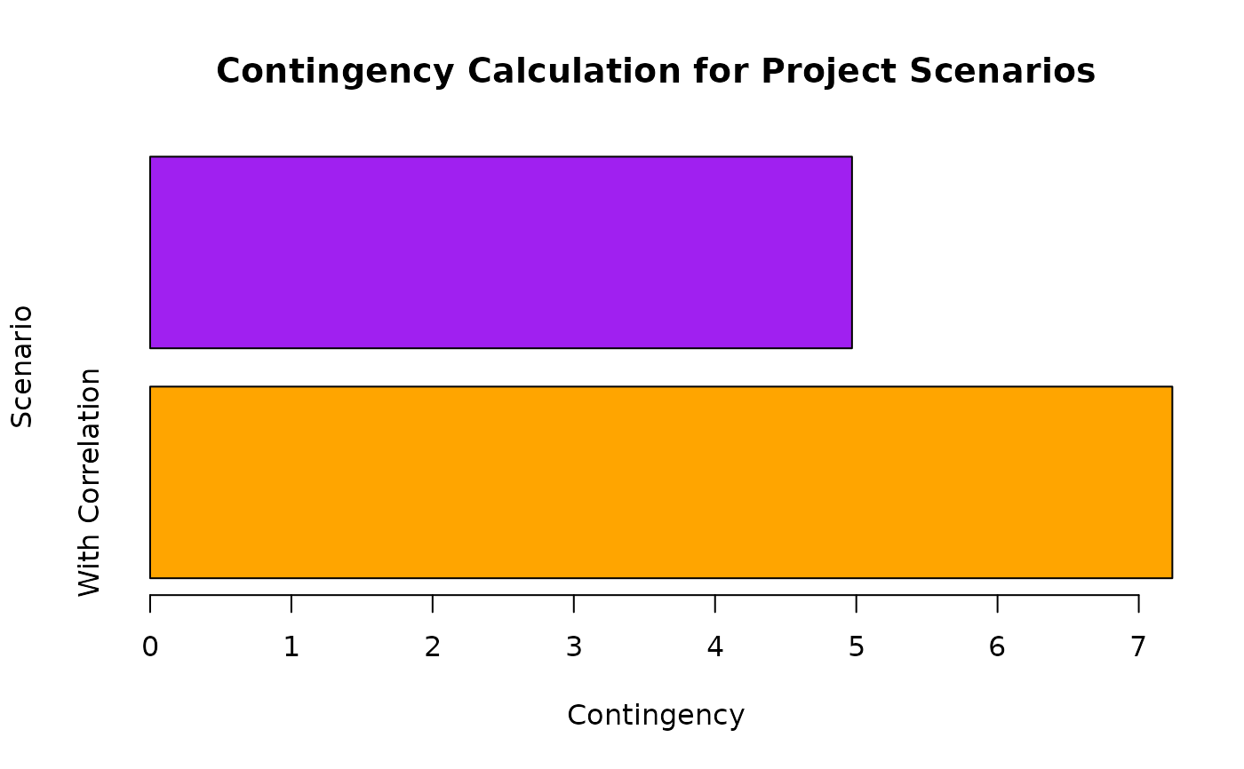
cat("Contingency based on 95th percentile and 50th percentile:", contingency)
#> Contingency based on 95th percentile and 50th percentile: 7.237666

# Without correlation matrix
results_indep <- mcs(num_sims, task_dists)
contingency_indep <- contingency(results_indep,
  phigh = 0.95,
  pbase = 0.50
)
cat("Contingency based on 95th percentile and 50th percentile (
independent tasks):", contingency_indep)
#> Contingency based on 95th percentile and 50th percentile (
#> independent tasks): 4.969658

# Build a barplot to visualize the contingency results.
contingency_data <- data.frame(
  Scenario = c("With Correlation", "Independent Tasks"),
  Contingency = c(contingency, contingency_indep)
)
barplot(
  height = contingency_data$Contingency,
  names = contingency_data$Scenario,
  col = c("orange", "purple"),
  horiz = TRUE,
  xlab = "Contingency",
  ylab = "Scenario"
)
title("Contingency Calculation for Project Scenarios")

References

Damnjanovic, Ivan, and Kenneth Reinschmidt. Data analytics for engineering and construction project risk management. No. 172534. Cham, Switzerland: Springer, 2020.