Agentic Risk Analysis • PRA

Overview

PRA includes an AI agent framework with three routing modes for user input:

Input type	Route	Example
`/command`	Deterministic — executes the tool directly, no LLM	`/mcs tasks=[...]`
Numerical data for computation	LLM tool call — the model selects and calls the right tool	“Simulate 3 tasks: Normal(10,2)…”
Conceptual / explanatory question	RAG — answered from the knowledge base, no tool call	“What is earned value?”

Three interfaces are available:

Slash commands (/mcs, /evm, /risk, …) - deterministic tool calls that bypass the LLM for instant, reliable results
Chat interface (pra_chat()) - programmatic R chat object powered by ellmer where the LLM selects tools or answers from RAG
Shiny app (pra_app()) - browser-based experience combining all three modes, powered by shinychat

Prerequisites

Install Ollama

Download from https://ollama.com, then pull a model:

ollama serve
ollama pull llama3.2
ollama pull nomic-embed-text  # for RAG embeddings

Install R dependencies

install.packages(c("ellmer", "ragnar", "shiny", "bslib", "shinychat", "jsonlite"))

Slash Commands

Slash commands provide deterministic tool execution, no LLM required. Type /help to see all available commands, or /help <command> for detailed usage with argument descriptions and examples.

Available commands

library(PRA)
cat(PRA:::format_help_overview())

Getting help for a command

Each command includes argument specifications, defaults, and examples:

cat(PRA:::format_command_help("mcs", PRA:::pra_command_registry()$mcs))

Example: Monte Carlo simulation

Run a simulation for a 3-task project directly:

set.seed(42)
r <- PRA:::execute_command(
  '/mcs n=10000 tasks=[{"type":"normal","mean":10,"sd":2},{"type":"triangular","a":5,"b":10,"c":15},{"type":"uniform","min":8,"max":12}]'
)
cat(r$result)
#> Monte Carlo Simulation Results (n = 10,000):
#> 
#> Summary Statistics:
#>   Mean  29.9804
#>   SD    3.113
#>   Min   19.502
#>   Max   41.3892
#> 
#> Percentiles:
#>   P5   24.8726
#>   P10  26.0194
#>   P25  27.8881
#>   P50  29.9536
#>   P75  32.0796
#>   P90  33.9873
#>   P95  35.1014

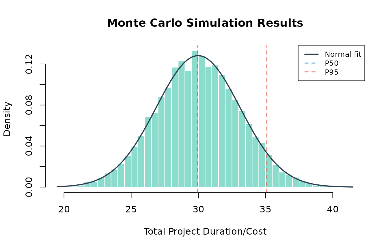
# The /mcs command stores results for chaining — visualize them:
result <- PRA:::.pra_agent_env$last_mcs
hist(result$total_distribution,
  freq = FALSE, breaks = 50,
  main = "Monte Carlo Simulation Results",
  xlab = "Total Project Duration/Cost",
  col = "#18bc9c80", border = "white"
)
curve(dnorm(x, mean = result$total_mean, sd = result$total_sd),
  add = TRUE, col = "#2c3e50", lwd = 2
)
abline(
  v = quantile(result$total_distribution, c(0.50, 0.95)),
  col = c("#3498db", "#e74c3c"), lty = 2, lwd = 1.5
)
legend("topright",
  legend = c("Normal fit", "P50", "P95"),
  col = c("#2c3e50", "#3498db", "#e74c3c"),
  lty = c(1, 2, 2), lwd = c(2, 1.5, 1.5),
  cex = 0.8, bg = "white"
)

Example: Chaining MCS to contingency

After running /mcs, chain to /contingency for the reserve estimate:

r <- PRA:::execute_command("/contingency phigh=0.95 pbase=0.50")
cat(r$result)
#> Contingency Analysis:
#> 
#>   Base Percentile      P50
#>   High Percentile      P95
#>   Contingency Reserve  5.1478

Example: Sensitivity analysis

Identify which tasks drive the most variance:

r <- PRA:::execute_command(
  '/sensitivity tasks=[{"type":"normal","mean":10,"sd":2},{"type":"triangular","a":5,"b":10,"c":15},{"type":"uniform","min":8,"max":12}]'
)
cat(r$result)
#> Sensitivity Analysis (variance contribution per task):
#> 
#>   Task 1    1
#>   Task 2    1
#>   Task 3    1

Example: Earned Value Management

Full EVM analysis with a single command:

r <- PRA:::execute_command(
  "/evm bac=500000 schedule=[0.2,0.4,0.6,0.8,1.0] period=3 complete=0.35 costs=[90000,195000,310000]"
)
cat(r$result)
#> Earned Value Management Analysis:
#> 
#> Core Metrics:
#>   Planned Value (PV)  300,000
#>   Earned Value (EV)   175,000
#>   Actual Cost (AC)    310,000
#> 
#> Variances:
#>   Schedule Variance (SV)  -125,000
#>   Cost Variance (CV)      -135,000
#> 
#> Performance Indices:
#>   Schedule Performance Index (SPI)  0.5833
#>   Cost Performance Index (CPI)      0.5645
#> 
#> Forecasts:
#>   EAC (Typical)                 885,714.3
#>   EAC (Atypical)                635,000
#>   EAC (Combined)                1,296,939
#>   Estimate to Complete (ETC)    575,714.3
#>   Variance at Completion (VAC)  -385,714.3
#>   TCPI (to meet BAC)            1.7105

Example: Bayesian risk probability

Calculate prior risk from two root causes:

r <- PRA:::execute_command(
  "/risk causes=[0.3,0.2] given=[0.8,0.6] not_given=[0.2,0.4]"
)
cat(r$result)
#> Bayesian Risk Analysis (Prior):
#> 
#>   Risk Probability  0.82
#>   Risk Percentage   82%
#>   Number of Causes  2

Then update with observations — Cause 1 occurred, Cause 2 unknown:

r <- PRA:::execute_command(
  "/risk_post causes=[0.3,0.2] given=[0.8,0.6] not_given=[0.2,0.4] observed=[1,null]"
)
cat(r$result)
#> Bayesian Risk Analysis (Posterior):
#> 
#>   Posterior Risk Probability  0.6316
#>   Posterior Risk Percentage   63.16%
#> 
#> Observations:
#>   Cause 1: Occurred
#>   Cause 2: Unknown

Example: Second Moment Method

Quick analytical estimate without simulation:

r <- PRA:::execute_command("/smm means=[10,12,8] vars=[4,9,2]")
cat(r$result)
#> Second Moment Method Results:
#> 
#>   Total Mean      30
#>   Total Variance  15
#>   Total Std Dev   3.873

Input validation and guidance

Missing or invalid arguments produce helpful error messages:

# Missing required arguments
r <- PRA:::execute_command("/risk causes=[0.3]")
cat(r$result)
#> **Missing required argument(s):** given, not_given
#> 
#> ### /risk — Bayesian Risk (Prior)
#> 
#> Calculate prior risk probability from root causes using Bayes' theorem.
#> 
#> **Arguments:**
#> - **causes** *(required)* — JSON array of cause probabilities, e.g. [0.3, 0.2]
#> - **given** *(required)* — JSON array of P(Risk | Cause), e.g. [0.8, 0.6]
#> - **not_given** *(required)* — JSON array of P(Risk | not Cause), e.g. [0.2, 0.4]
#> 
#> **Examples:**
#>   /risk causes=[0.3,0.2] given=[0.8,0.6] not_given=[0.2,0.4]

# Unknown command
r <- PRA:::execute_command("/simulate")
cat(r$result)
#> Unknown command: **/simulate**
#> 
#> Did you mean one of these?
#> - /mcs
#> - /smm
#> - /contingency
#> - /sensitivity
#> - /evm
#> - /risk
#> - /risk_post
#> - /learning
#> - /dsm
#> 
#> Type `/help` for a list of all commands.

Chat Interface

The chat interface routes queries through the LLM, which decides whether to call a tool or answer from RAG context:

Numerical data (distributions, costs, schedules) → LLM calls the appropriate tool and interprets the results
Conceptual questions (“what is CPI?”, “how does MCS work?”) → LLM answers from RAG knowledge base with source citations
Ambiguous → LLM uses RAG context and only calls a tool if data is present

library(PRA)
chat <- pra_chat(model = "llama3.2")

# Tool call: user provides numerical data
chat$chat("Run a Monte Carlo simulation for a 3-task project with
  Task A ~ Normal(10, 2), Task B ~ Triangular(5, 10, 15),
  Task C ~ Uniform(8, 12). Use 10,000 simulations.")

# RAG: conceptual question, no computation needed
chat$chat("What is the difference between SPI and CPI?")

For guaranteed reliability with computations, use /commands instead. The chat interface is best suited for exploratory questions and interpretation.

Using cloud models

For better accuracy with complex queries, supply a pre-configured ellmer chat object:

# OpenAI
chat <- pra_chat(chat = ellmer::chat_openai(model = "gpt-4o"))

# Anthropic
chat <- pra_chat(chat = ellmer::chat_anthropic(model = "claude-sonnet-4-20250514"))

Notes on chat reliability

Conceptual questions work well even with small models since they only require reading RAG context, not tool calling.
Tool calling quality depends on model size. llama3.2 (3B) handles simple single-tool queries; larger models (8B+) are more reliable for multi-step chains.
If the model attempts to call a tool for a conceptual question, or describes what it would do instead of calling tools, use /commands for deterministic results.

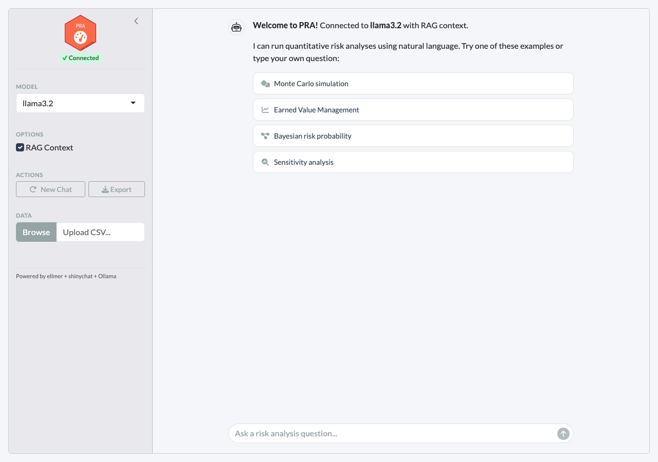
Interactive Shiny App

For a browser-based experience with streaming responses and inline visualizations:

pra_app()

The app supports all three input modes in the same chat panel:

Type /mcs tasks=[...] for instant deterministic results
Type “Simulate 3 tasks…” for LLM tool calling
Type “What is earned value?” for RAG-powered answers

Clicking an example prompt executes the /command instantly and displays rich results with tables and plots:

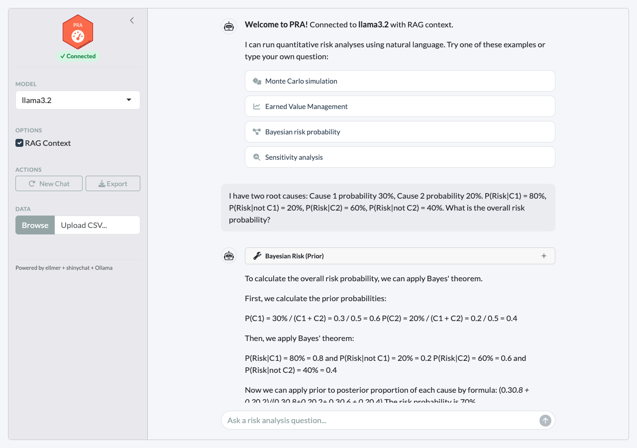
Features

Three input modes — /commands (deterministic), natural language (LLM tool calls), and conceptual questions (RAG)
Clickable example prompts that execute /commands on click
Streaming chat powered by shinychat with token-by-token responses
Inline tool results displayed as rich HTML tables and plots
RAG source citations — the agent cites knowledge base files for conceptual answers
Connection status badge showing model connectivity
Collapsible sidebar with model selection, RAG toggle, and CSV upload
Export — download the conversation as a markdown file

Configuration options

# Custom model and port
pra_app(model = "qwen2.5", port = 3838)

# Disable RAG for faster responses
pra_app(rag = FALSE)

RAG Knowledge Base

The agent is enhanced with domain knowledge through retrieval-augmented generation (RAG). When RAG context is retrieved, the agent cites the source files in its response.

Built-in knowledge files

File	Topics
`mcs_methods.md`	Distribution selection, correlation, interpreting percentiles
`evm_standards.md`	EVM metrics, performance indices, forecasting methods
`bayesian_risk.md`	Prior/posterior risk, Bayes’ theorem for root cause analysis
`learning_curves.md`	Sigmoidal models (logistic, Gompertz, Pearl), curve fitting
`sensitivity_contingency.md`	Variance decomposition, contingency reserves
`pra_functions.md`	PRA package function reference

How RAG context flows

User asks a question
The question is embedded and matched against the knowledge base using hybrid search (vector similarity + BM25)
The top 3 matching chunks are prepended to the query with [Source: filename] tags
The agent is instructed to cite these sources in its response
The agent uses the context to inform its answer while still calling tools for computation

Adding your own documents

store <- build_knowledge_base()

# Add a single file
add_documents(store, "path/to/my_risk_register.md")

# Add all .md and .txt files in a directory
add_documents(store, "path/to/project_docs/")

Disabling RAG

# Chat without RAG
chat <- pra_chat(model = "llama3.2", rag = FALSE)

# App without RAG
pra_app(rag = FALSE)

Available Commands and Tools

Slash commands (deterministic)

Command	Description
`/mcs`	Monte Carlo simulation with task distributions
`/smm`	Second Moment Method (analytical estimate)
`/contingency`	Contingency reserve from last MCS
`/sensitivity`	Variance contribution per task
`/evm`	Full Earned Value Management analysis
`/risk`	Bayesian prior risk probability
`/risk_post`	Bayesian posterior risk after observations
`/learning`	Sigmoidal learning curve fit and prediction
`/dsm`	Design Structure Matrix
`/help`	List all commands or get help for one

LLM tools (via chat)

Module	Tool	Use case
Simulation	`mcs_tool`	Full Monte Carlo with distributions
Analytical	`smm_tool`	Quick mean/variance estimate
Post-MCS	`contingency_tool`	Reserve at confidence level
Post-MCS	`sensitivity_tool`	Variance contribution per task
EVM	`evm_analysis_tool`	All 12 EVM metrics in one call
Bayesian	`risk_prob_tool`	Prior risk from root causes
Bayesian	`risk_post_prob_tool`	Posterior risk after observations
Bayesian	`cost_pdf_tool`	Prior cost distribution
Bayesian	`cost_post_pdf_tool`	Posterior cost distribution
Learning	`fit_and_predict_sigmoidal_tool`	Pearl/Gompertz/Logistic
DSM	`parent_dsm_tool`	Resource-task dependencies
DSM	`grandparent_dsm_tool`	Risk-resource-task dependencies

Evaluation with vitals

PRA includes an evaluation framework for measuring LLM tool-calling accuracy using the vitals package. The evaluation suite in inst/eval/pra_eval.R tests 15 scenarios across three tiers:

Tier	Description	Example
Single-tool	One tool call	“Simulate 3 tasks with distributions…”
Multi-tool chain	Sequential tool calls	“Run MCS then calculate contingency at 95%”
Open-ended	Requires interpretation	“My project is behind schedule, here’s EVM data…”

# Run evaluation
source(system.file("eval/pra_eval.R", package = "PRA"))
results <- run_pra_eval(model = "llama3.2")

# Compare models
comparison <- run_pra_comparison(
  models = c("llama3.2", "qwen2.5"),
  rag_options = c(TRUE, FALSE)
)

Troubleshooting

Tool calling not working

Small models sometimes describe what they would do rather than actually calling tools. Use /commands for reliable deterministic execution:

# Instead of asking the LLM:
chat$chat("Run a Monte Carlo simulation...")

# Use the /command directly in the app:
# /mcs tasks=[{"type":"normal","mean":10,"sd":2}]

Other workarounds for LLM chat:

Use llama3.1 (8B) or larger for better tool calling than 3B models
Be explicit: “Call the mcs_tool with these parameters…”
Use a cloud model: pra_chat(chat = ellmer::chat_openai(model = "gpt-4o"))

Slow responses

Use a smaller model (llama3.2 is 3B, faster than llama3.1 8B)
Ensure GPU acceleration is active (ollama ps)
Disable RAG if not needed: pra_chat(rag = FALSE)
Use /commands — they execute instantly without LLM overhead

RAG build fails

install.packages("ragnar")

ollama pull nomic-embed-text

Source citations missing

If the agent does not cite sources in RAG-enabled responses, try:

Using a larger model (8B+ models follow citation instructions more reliably)
Being explicit: “Cite your sources in the response”