Repairable Systems Analysis

Introduction

Repairable systems are systems that can be restored to a functioning state after a failure. Unlike non-repairable items where we model time-to-first-failure, repairable systems generate recurrent events – a sequence of failure times over the system’s life. The Non-Homogeneous Poisson Process (NHPP) provides a natural framework for modeling these recurrence patterns.

ReliaGrowR provides four key tools for analyzing repairable systems:

1. mcf() – Non-parametric Mean Cumulative Function estimation
2. exposure() – Exposure analysis (total operating time at risk)
3. nhpp() – Parametric NHPP model fitting (Power Law and Log-Linear)
4. predict_nhpp() – Forecasting future events from a fitted model

Mean Cumulative Function

The Mean Cumulative Function (MCF) is a non-parametric estimate of the expected cumulative number of events per system over time. It makes no assumptions about the underlying process and is useful as an exploratory tool before fitting parametric models.

For a fleet of systems, the MCF at time $t$ is estimated using the Nelson-Aalen estimator:

$$\hat{M}(t) = \sum_{t_j \le t} \frac{d_j}{n_j}$$

where $d_j$ is the number of events at time $t_j$ and $n_j$ is the number of systems still under observation.

Example

Consider three systems with the following event histories:

library(ReliaGrowR)

id   <- c(1, 1, 1, 2, 2, 2, 3, 3, 3, 3)
time <- c(100, 350, 500, 80, 300, 600, 150, 250, 400, 700)

Compute and plot the MCF:

result <- mcf(id, time)
plot(result, main = "Mean Cumulative Function",
     xlab = "Time", ylab = "MCF")

The step-function plot shows the estimated average cumulative events per system over time, with dashed confidence bounds.

Using Data Frames

The mcf() function also accepts a data frame:

df <- data.frame(id = id, time = time)
result2 <- mcf(data = df)

Censored Observations

If some systems are withdrawn from observation before the end of the study, use the event indicator (1 = event, 0 = censored):

id    <- c(1, 1, 1, 2, 2, 2, 3, 3, 3)
time  <- c(100, 350, 500, 80, 300, 400, 150, 250, 700)
event <- c(  1,   1,   0,  1,   1,   0,   1,   1,   1)

result <- mcf(id, time, event)

System 1 was censored at time 500 and System 2 at time 400. The MCF accounts for the reduced number of systems at risk after these times.

Exposure-Adjusted MCF

When systems are observed beyond their last event time (i.e., the system was running but no event occurred), it is important to specify the actual end-of-observation time. Otherwise, the MCF assumes a system left observation at its last event, which inflates the estimated recurrence rate.

The end_time parameter specifies the actual observation window per system:

id   <- c(1, 1, 2, 2, 3, 3)
time <- c(100, 300, 150, 400, 200, 350)

# Without end_time: system observation ends at last event
mcf_basic <- mcf(id, time)

# With end_time: all systems observed until time 800
mcf_adj <- mcf(id, time, end_time = c("1" = 800, "2" = 800, "3" = 800))

Compare the two MCF estimates:

par(mfrow = c(1, 2))
plot(mcf_basic, main = "MCF (inferred exposure)",
     xlab = "Time", ylab = "MCF")
plot(mcf_adj, main = "MCF (explicit exposure)",
     xlab = "Time", ylab = "MCF")

The exposure-adjusted MCF produces lower estimates because all three systems remain in the risk set for the full observation period – even at times beyond their last event.

Using Exposure Results with MCF

The exposure() function returns per-system end-of-observation times in its end_times field, which can be passed directly to mcf():

id    <- c(1, 1, 1, 2, 2, 2, 3, 3, 3)
time  <- c(100, 350, 500, 80, 300, 400, 150, 250, 700)
event <- c(  1,   1,   0,  1,   1,   0,   1,   1,   1)

exp_result <- exposure(id, time, event)
mcf_result <- mcf(id, time, event, end_time = exp_result$end_times)

This workflow ensures the MCF and exposure calculations use the same observation windows.

Exposure Analysis

Exposure measures the total operating time during which events can occur across all systems in a fleet. It is fundamental to repairable systems analysis because event rates are only meaningful when normalized by the time during which events could have been observed.

For $k$ systems observed up to times $T_1, T_2, \ldots, T_k$, the total exposure is:

$$E = \sum_{i=1}^{k} T_i$$

The cumulative exposure at time $t$ is:

$$E(t) = \sum_{i=1}^{k} \min(t, T_i)$$

Each system contributes time up to the lesser of $t$ or its observation end. The event rate is then $r(t) = N(t) / E(t)$, the cumulative number of events per unit exposure.

Example

Using the same three-system fleet from the MCF example:

id   <- c(1, 1, 1, 2, 2, 2, 3, 3, 3, 3)
time <- c(100, 350, 500, 80, 300, 600, 150, 250, 400, 700)
result <- exposure(id, time)

The exposure() function returns a table showing, at each event time, the number of systems at risk, cumulative exposure, cumulative events, and the event rate.

Multi-Panel Plot

The default plot method produces a three-panel dashboard:

plot(result)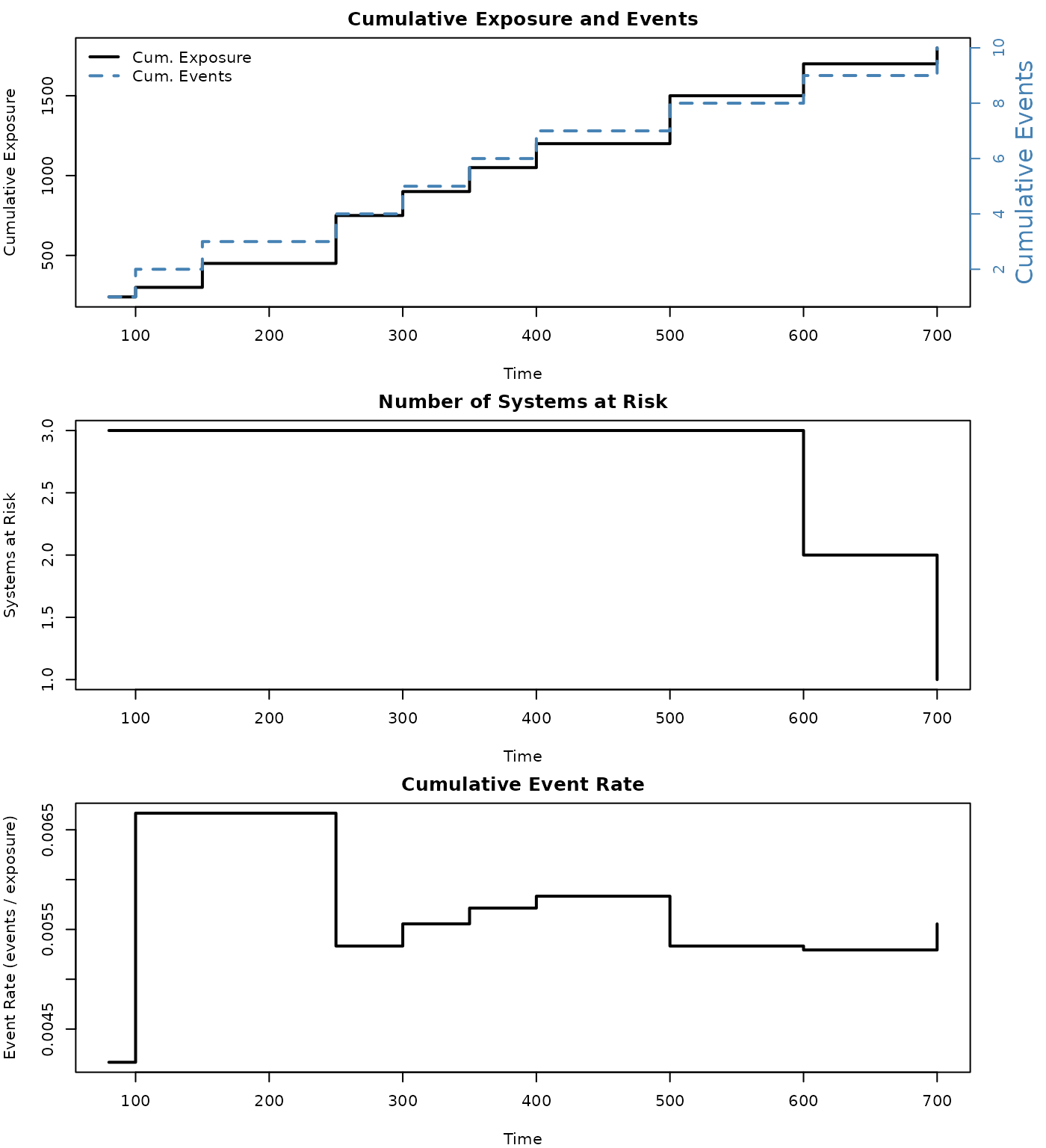

The top panel shows cumulative exposure (left axis) and cumulative events (right axis, blue). The middle panel tracks the number of systems under observation. The bottom panel shows the cumulative event rate (events per unit exposure).

Single Panel Plots

Individual panels can be selected with the which argument:

plot(result, which = "exposure")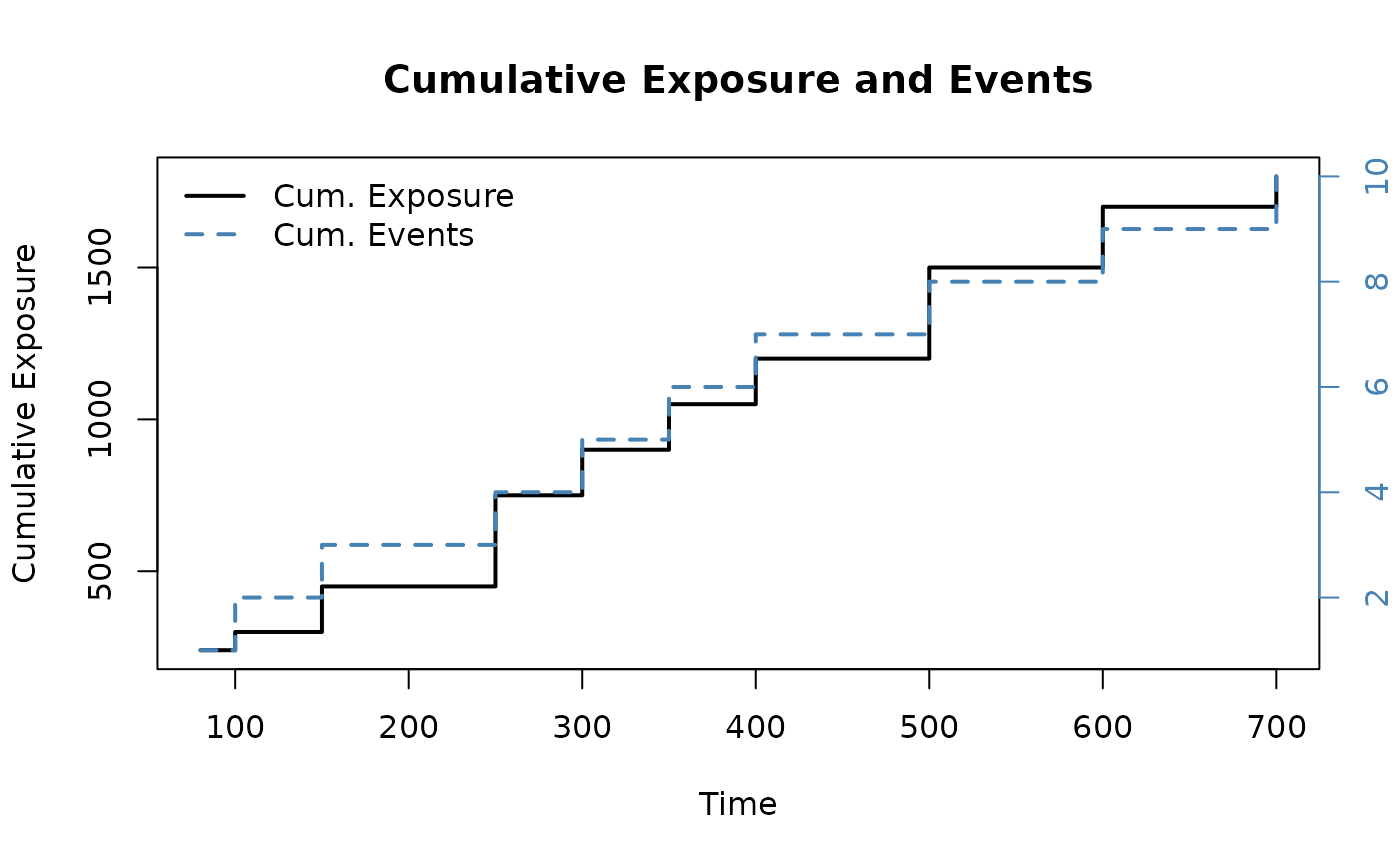

plot(result, which = "event_rate")

Exposure with Censoring

When systems are withdrawn before the end of study, their observation time still contributes to exposure up to the censoring point:

id    <- c(1, 1, 1, 2, 2, 2, 3, 3, 3)
time  <- c(100, 350, 500, 80, 300, 400, 150, 250, 700)
event <- c(  1,   1,   0,  1,   1,   0,   1,   1,   1)

result <- exposure(id, time, event)

System 1 (censored at 500) and System 2 (censored at 400) contribute exposure up to their respective censoring times, but only actual events are counted in the cumulative event tally.

Power Law NHPP

The Power Law NHPP models the cumulative number of events as:

$$N(t) = \lambda\, t^{\beta}$$

The parameter $\beta$ indicates the trend:

• $\beta > 1$: deteriorating system (increasing event rate)
• $\beta = 1$: constant rate (Homogeneous Poisson Process)
• $\beta < 1$: improving system (decreasing event rate)

Example

time  <- c(200, 400, 600, 800, 1000, 1200, 1400, 1600, 1800, 2000)
event <- c(  3,   5,   4,   7,    6,    8,    5,    9,    7,   10)

Fit using Maximum Likelihood Estimation (default):

fit_mle <- nhpp(time, event, method = "MLE")
plot(fit_mle, main = "Power Law NHPP (MLE)",
     xlab = "Cumulative Time", ylab = "Cumulative Events")

Fit using Least Squares:

fit_ls <- nhpp(time, event, method = "LS")

Both methods estimate similar parameters. MLE is generally preferred for its statistical properties, while LS provides a simple regression-based approach and supports piecewise models.

Log-Linear NHPP

The Log-Linear NHPP models the event intensity as:

$$\lambda(t) = \exp(a + bt)$$

with cumulative function:

$$\Lambda(t) = \frac{e^a}{b}\left(e^{bt} - 1\right)$$

The parameter $b$ controls the trend: $b > 0$ means an increasing rate, $b < 0$ a decreasing rate, and $b \approx 0$ a constant rate.

Example

result_ll <- nhpp(time, event, model_type = "Log-Linear")
plot(result_ll, main = "Log-Linear NHPP",
     xlab = "Cumulative Time", ylab = "Cumulative Events")

Segmented NHPP

The Piecewise Power Law NHPP allows different parameters in different time segments. This is useful when a system’s behavior changes – for example, after a major overhaul or design change.

With User-Specified Breakpoints

time  <- c(100, 200, 300, 400, 500, 600, 700, 800, 900, 1000,
           1100, 1200, 1300, 1400, 1500)
event <- c(  1,   1,   2,   4,   4,   1,   1,   2,   1,    4,
             1,   1,   3,   3,   4)

result_pw <- nhpp(time, event, breaks = c(500), method = "LS")
plot(result_pw, main = "Piecewise Power Law NHPP",
     xlab = "Cumulative Time", ylab = "Cumulative Events")

The vertical dashed line indicates the change point at time 500. Each segment has its own $\beta$ and $\lambda$ parameters.

Forecasting

The predict_nhpp() function forecasts cumulative events at future times using a fitted NHPP model.

Example

time  <- c(200, 400, 600, 800, 1000, 1200, 1400, 1600, 1800, 2000)
event <- c(  3,   5,   4,   7,    6,    8,    5,    9,    7,   10)

fit <- nhpp(time, event, method = "MLE")
fc <- predict_nhpp(fit, time = c(2001, 2500, 3000, 4000, 5000))

Plot the observed data with the forecast:

plot(fc, main = "NHPP Forecast",
     xlab = "Cumulative Time", ylab = "Cumulative Events")

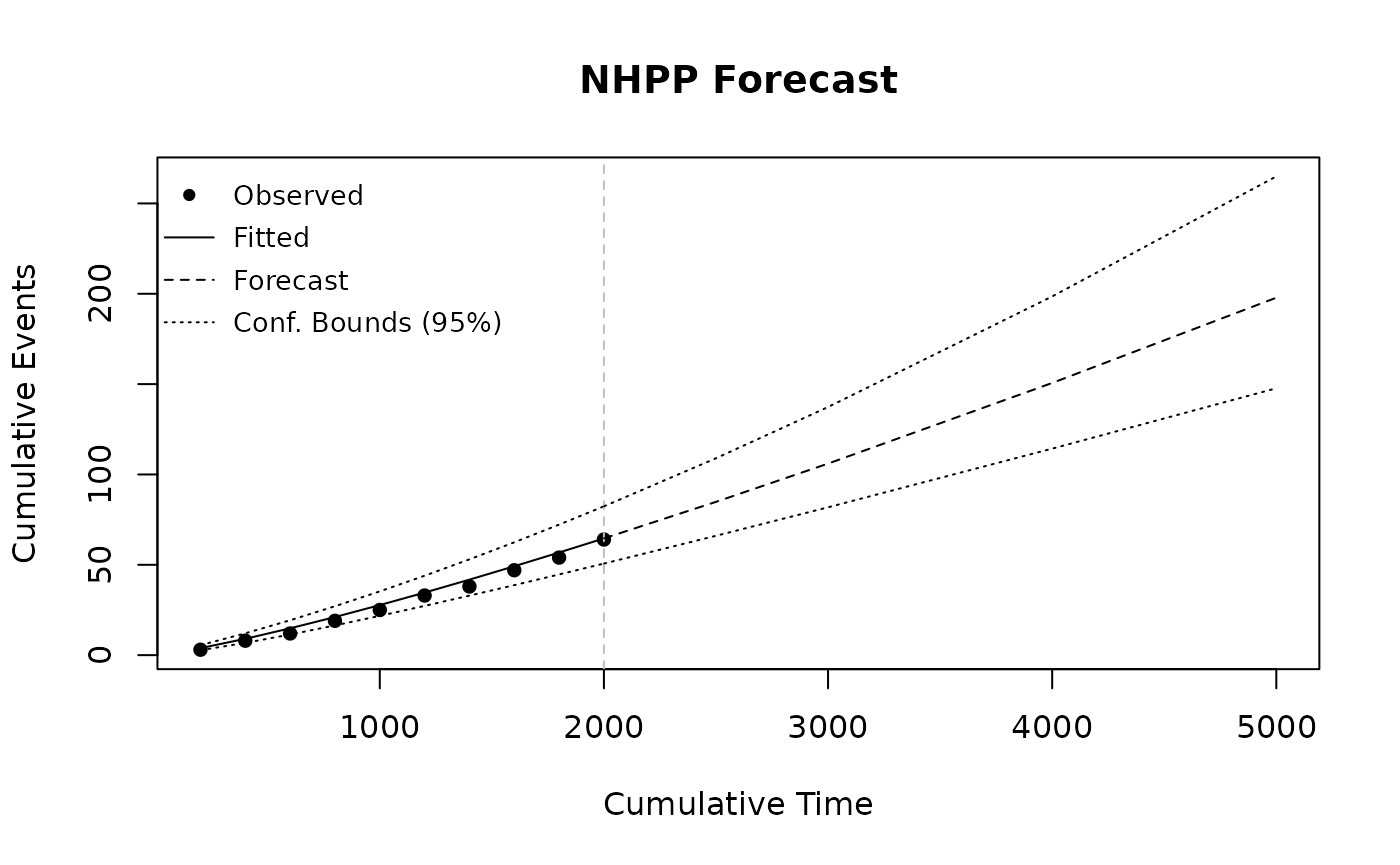
The plot shows the observed data (points), the fitted model (solid line), and the forecast (dashed line) with confidence bounds. The vertical gray line marks the boundary between observed and forecast periods.

Forecasting also works with Log-Linear models:

fit_ll <- nhpp(time, event, model_type = "Log-Linear")
fc_ll <- predict_nhpp(fit_ll, time = c(2500, 3000))

Summary

NHPP models provide a flexible framework for analyzing repairable systems:

• The MCF gives a non-parametric view of the recurrence pattern, useful for exploratory analysis and comparing systems.
• Exposure analysis quantifies the total time at risk and event rates, providing essential context for interpreting event counts.
• The Power Law NHPP is the most widely used parametric model, with $\beta$ directly indicating whether the system is improving or deteriorating.
• The Log-Linear NHPP offers an alternative parametric form for modeling time-dependent intensity.
• Piecewise models capture changes in system behavior across different operational phases.
• Forecasting with predict_nhpp() supports planning for spare parts, maintenance scheduling, and warranty analysis.